Fitting parameters of a simple process model (optimisation & uncertainty)

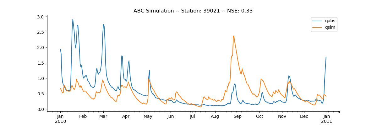
I have a very simple hydrological model. The model can be simply conceptualised as below:

Simple Hydro model 492x394

I am trying to learn the values of the parameters a, b and c.

Where:

P = Precipitation Inputs
L = Losses 
S = Storage (groundwater / soil)
Qf = Fast Flow
Qs = Slow Flow

a = Proportion of P[t] passing into S[t]
b = Proportion of P[t] lost (e.g. to evaporation)
c = Proportion of S[t] passing into Qs[t] (slow flow)

The equations are:

Q[t] = Qf[t] +Qs[t]
Qs[t] = S[t] * c
Qf[t] = P[t] * (1 - a - b)
S[t] = S[t - 1] * (1 - c) + (P[t] * a)
L[t] = P[t] * b

In python this model looks like this:

def abcmodel(
    P: float,
    S: float,
    a: float,
    b: float,
    c: float,
) -> Tuple[float, float]:
    """Modelling flow using ABC model

    Args:
        P (float): Precipitatio
        S (float): Storage (groundwater / soil)
        a (float): proportion of precipitation into storage bounds: 0-1
        b (float): proportion of precipitation lost bounds: 0-1
        c (float): proportion of storage becoming low flow bounds: 0-1

    Returns:
        Q (float): discharge
        S (float): storage
    """
    L = b * P
    Qf = (1 - a - b) * P
    Qs = c * S
    dsdt = (a * P) - (c * S)
    Q = Qf + Qs
    return Q, dsdt


def run_abcmodel(
    initial_state: float,
    precip: np.ndarray,
    a: float,
    b: float,
    c: float,
):
    num_timesteps: int = len(precip)

    # intialize arrays to store values
    qsim = np.zeros(num_timesteps, np.float64)
    storage = np.zeros(num_timesteps, np.float64)

    # initialize inital state (storage)
    storage[0] = initial_state

    for t in range(1, num_timesteps):
        # run the simulations
        Q, dsdt = abcmodel(
            P=precip[t],
            S=storage[t - 1],
            a=a,
            b=b,
            c=c
        )

        # Calculate the streamflow
        qsim[t] = Q

        # Update the storage
        storage[t] = storage[t - 1] + dsdt

    return qsim, storage

(see below for a working example of the python code).

I want to use Stan to optimise the parameters and get uncertainty estimates of their values.

Longer term I want to add complexity by including observation error (in Q) and process error (from the ABC model).

My stan code is looking something like this (with gaps - sorry!)

functions{
    real[] abcmodel(
        real a,
        real b,
        real c,
        real[] precip,
        real[] S,
    ){
        # do i want to return dsdt
        # dsdt[i] = (a * P[i]) - (c * S[i - 1])

        # but S is unobserved?
        # Q is observed so I want to return a simulated Q ?
    }
}
data{
    int<lower=0> T;
    real Q[T];
    real P[T];
}
parameters{
    real<lower=0, upper=1> a;
    real<lower=0, upper=1> b;
    real<lower=0, upper=1> c;
}
model{
    real qsim[T];
    real S[T];

    # do I want to use `integrate_ode_rk45` ?
}

Any help is very much appreciated!

Current code:
Here is a working python example of the model with a method for selecting the parameters (Using - scipy.optimize.differential_evolution)
abcmodel_example.py (4.0 KB)

Here’s the attempted cmdstanpy file
cmdstanpy_attempt1.py (837 Bytes)

And the stan attempt
abcmodel.stan (563 Bytes)

Have you taken a look at some of the case studies?

I found @Bob_Carpenter’s case studies to be very helpful in getting me started with coding ODE models. See https://mc-stan.org/users/documentation/case-studies/soil-knit.html

Since Q is observed, as is indicated by your data block, indeed, you will want to return a vector of simulated Q’s. You will need that for your likelihood that is written up in the model data block.

model {
...
obs_Q ~ normal(sim_Q, sigma)
}

assuming normal measurement error.

With respect to your question for which integrator to use, do you know how stiff your system is? Stan does have two non-stiff integrators at this point in rk45 and Adams-Moulton. There is one stiff option in the CVODE implementation of BDF.

Also, is P[T]a vector of observations that you will want to use for fitting in addition to Q[T]? Are you intending to fit bivariate data?

1 Like

Thanks @xiehw really appreciate the help!

1) Stiff system?
If I’m honest I am not certain what a stiff system is. From my brief glance at Wikipedia I don’t think it’s a particularly sensitive system and so I would say it’s not stiff.

2) Univariate / Bivariate Model

So P_t is the input / forcing data for the process model. I don’t think i want to fit a bivariate model. My understanding is that I am currently observing the discharge. Eventually, in a more complex model, we also observe (very noisily) the soil moisture / storage (S_t).

3) Stan Case Study

I had not seen that case study, thanks so much for sharing! I hadn’t checked the case studies before 2016. I am just writing the system below in the same format as the case study.

The system dynamics are modelled through:
Q_t = Qf_t + Qs_t
Qf_t = (1-a-b) P_t
Qs_t = c S_t
S_t = (1-c) S_{t-1} + aP_t
L_t = bP_t

Where:
Q_t = River Flow
Qf_t = Fast Flow
Qs_t = Slow Flow
S_t = Storage
L_t = Losses

I want to solve the equations for Q_{t} at measurement times t = {1, ..., T}

My updated stan code is here:

functions{
    // System state S is one dimensional storage
    // The evolution of S is determined by 2 parameters
    //  a: proportion of Precipitation (P) to Storage (S)
    //  c: Proportion of Storage (S) to Slow Flow (Qs)
    // And driven by the changes in
    //  P: precipitation inputs
    real[] ode_abcmodel_state(
        real t,
        real P,
        real[] S,
        real[] theta;
        real[] x_r;
        real[] x_i;
    ){
        real a;
        real b;
        real dSdt;

        a = theta[1];
        b = theta[2];

        dSdt = (a * P) - (c * S);

        return dSdt;
    }

    /**
    * ABC Hydrological Model
    * Compute total simulated flow from the system given
    *  parameters and times. This is done by simulating
    *  the system storage defined in ode_abcmodel_state
    *
    * Parameters:
    * ----------
    *  @param T : number of times
    *  @param t0: initial time
    *  @param ts: observation times
    *  @param P: observation for Precipitation
    *  @param a : proportion of Precipitation (P) to Storage (S)
    *  @param b : proportion of Precipitation (P) lost to evaporation
    *  @param c : Proportion of Storage (S) to Slow Flow (Qs)
    *  @return Q: evolved discharge for times ts
    */
    real[] abcmodel(
        int T;
        real t0;
        real[] ts;
        real[] P,
        real a;
        real b;
        real c;
        real[] x_r;
        real[] x_i;
    ){
        real S_t0;          // initial state
        real theta[3];      // ABCModel parameters
        real S_hat[T];      // predicted Storage content
        real Qsim[T];       // simulated flow

        // initialise parameters
        theta[1] = a;
        theta[2] = b;
        theta[3] = c;

        // integrate the system
        // HOW TO PASS IN P[t] ??
        S_hat = integrate_ode_rk45(
            ode_abcmodel_state,
            S_t0, t0, ts, theta
        );

        # calculate system evolution over time
        for (t in 1: T)
            S[t] = ((1 - c) * S_hat[t - 1]) + (a * P[t]);
            Qs[t] = c * S[t];
            // L[t] = b * P[t]
            Qf[t] = (1 - a - b) * P[t];
            Qsim[t] = Qf[t] + Qs[t];

        return Qsim;
    }

}
data{
    int<lower=0> T;
    real Q[T];      // measured flow
    real P[T];      // measured precipitation
    real S_t0;      // initial storage
}
transformed data{
    // Why are these here? Copied from example
    real x_r[0];    // no real data for ODE system
    int x_i[0];     // no integer data for ODE system
}
parameters{
    real<lower=0, upper=1> a;
    real<lower=0, upper=1> b;
    real<lower=0, upper=1> c;
    real<lower=0, upper=1> sigma;
}
transformed parameters{
    real Qsim[T];   // process model for flow (Q)

    Qsim = abcmodel(
        T, t0, ts, P, a, b, c, x_r, x_i
    );
}
model{
    // Priors
    // What priors to choose?
    a ~ normal(0.5, 1);
    b ~ normal(0.5, 1);
    c ~ normal(0.5, 1);
    sigma ~ normal(0, 1);

    # normal measurement error of Q
    for (t in 1: T)
        Q[t] ~ normal(sim_Q[t], sigma);
}

Some questions:

  • What are x_r and x_i, vectors passed to the ode_abcmodel_state function (and the two_pool_feedback function in the example)?
  • How do I pass the Precipitation vector (P[t]) into the ode_abcmodel_state function?
  • How should I think about the difference between ode_abcmodel_state and abcmodel. Are these implemented correctly?
  • What priors would be sensible starting points, the only real information I have is the bounds between 0-1 given that this is a highly idealised system. Although c is likely much smaller than a, b.

Before getting into the priors, it looks like you have a delay differential equation (DDE) system with a discrete delay. You may definitely know more than me here, so do correct me if I’m wrong (I’m not used as much to that style of notation for ODEs, as in my field \frac{dy}{dt} is used more often, but I think I do have some bad news here – you need DDE integration to solve that system because of the expression in S_t. I am really not familiar with DDEs, but Stan does not have a DDE integrator. However, I think you can still do this with a low accuracy explicit Euler method if you have information for t = 0 and t = 1. That said, is your system a difference equation rather than a set of differential equations? I have seen notation like this for difference equations. Difference equations, you solve through by just looping through the times, and then you would not use differential equation integrators at all.

So right now, there is no way of passing in forcing vectors into Stan. Constants and forcing elements must be passed in individually. x_r is for reals, while x_i is the container for integers. However, this will soon be changed due to the work that folks including @bbbales2, @wds15, and @rok_cesnovar are doing, so vectors will be able to be directly passed into ODE functions, and there will be more freedom in defining the arguments for ODE functions.

I do have a suspicion now that your system is a system of difference equations (http://www.eco.uc3m.es/~rimartin/Teaching/AMATH/NOTES2EN.pdf) because of the notation. If I’m wrong, and this is a system of differential equations, a self-coded Euler method perhaps should be attempted.

Interesting! I think it might be a difference equation for this simple model. I was hoping that adding in complexity (for example when we have two stores like in the soil carbon example) would be easier to build up from this simple case.

I guess some of the confusion comes from the fact that the modelled quantity (Q_t) is not a function of (Q_{t-1}). Q_t is a function of P_t and S_t). That’s why i wondered whether I needed to incorporate the change in S_t which is a function of S_{t-1}.

S_t = (1 - c)S{t-1} + aP_t

If it is just a simple loop does that make it easier? Then I could have something like:

data{
    int<lower=0> T;
    real Q[T];      // measured flow
    real P[T];      // measured precipitation
    real S_t0;      // initial storage
}

parameters{
    real<lower=0, upper=1> a;
    real<lower=0, upper=1> b;
    real<lower=0, upper=1> c;
    real<lower=0, upper=1> sigma;
}

transformed parameters{
    real Qsim[T];
    real Qs[T];
    real Qf[T];
    real S[T];

    // process model for flow (Q)
    S[1] = S_t0;     // Set the initial estimate of the storage
    for (t in 2:T){
        S[t] = ((1 - c) * S[t - 1]) + (a * P[t]);
        Qs[t] = c * S[t];
        Qf[t] = (1 - a - b) * P[t];
        Qsim[t] = Qf[t] + Qs[t];
    }
}

model{
    // Priors
    a ~ normal(0.5, 1);
    b ~ normal(0.5, 1);
    c ~ normal(0.5, 1);
    sigma ~ normal(0, 1);


    // normal measurement error of Q
    for (t in 1: T)
        Q[t] ~ normal(Qsim[t], sigma);
}

However, this model does not (yet) compile.

I think a lot of the confusion comes from not being fully aware of the tool required. What I do know is that I want to use the power of HMC for sampling the parameters of the model, and then incorporate measurement uncertainty on top of the process model.

Thanks so much for your links, these are incredibly useful resources!

Tommy

1 Like

Yep, for solving a difference equation, a loop will be the way to go about it. Glad we got the difference/differential equation distinction classified! A difference equation model is still possible to code up in Stan. It looks like your code is on the right track. I would think that you probably need to initialize values for Qsim0, Qs0, and Qf0 alongside S_t0? And for your likelihood loop, you may want to start that loop from t = 2.

What you are trying to do looks similar to some of my own current work, which draws heavily from Bob Carpenter’s case studies. There is a pre-print describing one project that is under review here: https://www.biogeosciences-discuss.net/bg-2020-23/. The project was one consisting of differential equation model comparison, but you may still find both the pre-print supplement and code (OSF | A Bayesian Approach to Evaluation of Soil Biogeochemical Models Meta-analysis Data and R and Stan Code) useful, as I definitely had to hack around with a few things to make them work.

1 Like

One thing that I am trying to understand a bit more is how to incorporate both measurement error and process error. In this model there will be A LOT of process error. Where would I incorporate error in the process?

Would I have to move the ABCModel process-model statements:

transformed parameters{
    real Qsim[T];
    real Qs[T];
    real Qf[T];
    real S[T];

    // process model for flow (Q)
    S[1] = S_t0;     // Set the initial estimate of the storage
    for (t in 2:T){
        S[t] = ((1 - c) * S[t - 1]) + (a * P[t]);
        Qs[t] = c * S[t];
        Qf[t] = (1 - a - b) * P[t];
        Qsim[t] = Qf[t] + Qs[t];
    }
}

From the transformed parameters to the model block?

Would it work by adding an error term epsilon to the State update equation?

parameters{
    ...
    real epsilon;
}

transformed parameters{
    ...
    S[1] = S_t0;     // Set the initial estimate of the storage
    for (t in 2:T){
        S[t] = ((1 - c) * S[t - 1]) + (a * P[t]) + epsilon;
        Qs[t] = c * S[t];
        Qf[t] = (1 - a - b) * P[t];
        Qsim[t] = Qf[t] + Qs[t];
}

model{
     // priors
     ....
     epsilon ~ normal(0, 1)
}

Because ultimately I would be interested in modelling the errors in the process-model using a Gaussian Process.

Thanks for sharing that code! It’s so useful to have a suite of stan models to look through and put something together!

I’m not familiar enough with GPs or process errors unfortunately to comment on that for now; do you have a link to a paper that the model is from or based on that could provide some more background information about the process error?

I hope one person more familiar than me with process error sees this thread; sorry I couldn’t be more of help on this front!

For sure thanks so much!

What we’re trying to emulate is this paper (with a much simpler model to begin with).

They are looking at simulating soil moisture, whereas we are interested in predicting discharge (y_t = Q_t).

translating their notation:
f = our ABC model (a process-based model PBM)
\psi = the hybrid prediction model that combines f and the GP model (hybrid process based model HPBM)
v_t = the state vector

Ultimately, I was hoping to use this project to learn more about Stan, probabilistic programming and bayesian methods!

I can’t decide if my state vector should be:

  1. storage (unobserved), parameters abc, precipitation inputs and observed discharge, v_t = [S_t, a, b, c, P_t, Q_t])
  2. just the unobserved storage ( v_t = [S_t])

Initially I wanted to optimise the parameters to choose a, b, c.

But ultimately I am interested in replicating this approach for discharge - combining a GP model with the process based model. First using this simple process based model (ABC Model - see here for another explanation/overview - in the appendix!), but ideally using more complex models as we go on!

Links:
A Data Scientist’s Guide to Streamflow Prediction., Gauch and Lin 2020
Combining Parametric Land Surface Models with Machine Learning, Pelissier et al 2020

Having got the very simple optimisation working, the results do return similar values for the parameters as the Python code!

I fit the model on a single basin’s data, River Cherwell at Enslow Mill, Station: 39021.

I recover similar parameter estimates from both methods! Which is a start.

Original Scipy optimisation:

{
    'a': 0.31194221014291457, 
    'b': 0.6840453791323466, 
    'c': 0.07970196684016911
}

Stan optimisation:

{
    'a': 0.35479324825, 
    'b': 0.66791806375, 
    'c': 0.0694573388
}

download

Really appreciate you taking the time @xiehw . Might even be worth opening a different question if i can’t edit the original one!

1 Like

Great to hear! What error terms or implementations did you end up using?

1 Like

Stan code:

data{
    int<lower=0> T;
    real Q[T];      // measured flow
    real P[T];      // measured precipitation
    real S_t0;      // initial storage
}

parameters{
    real<lower=0, upper=1> a;
    real<lower=0, upper=1> b;
    real<lower=0, upper=1> c;
    real<lower=0, upper=1> sigma;
}

transformed parameters{
    real Qsim[T];
    real Qs[T];
    real Qf[T];
    real S[T];

    // process model for flow (Q)
    S[1] = S_t0;     // Set the initial estimate of the storage
    for (t in 2:T){
        S[t] = ((1 - c) * S[t - 1]) + (a * P[t]);
        Qs[t] = c * S[t];
        Qf[t] = (1 - a - b) * P[t];
        Qsim[t] = Qf[t] + Qs[t];
    }
}

model{
    // Priors
    a ~ normal(0.5, 1);
    b ~ normal(0.5, 1);
    c ~ normal(0.5, 1);
    sigma ~ normal(0, 1);

    // normal measurement error of Q
    for (t in 1: T)
        Q[t] ~ normal(Qsim[t], sigma);
}

Then the script to run the model and extract results is here (using cmdstanpy):
cmdstanpy_attempt1.py (2.3 KB)

I am surprised that the parameters are so certain, given that the model does such a poor job of simulating the observations.


|600px;x400px;

Like a year late to the river flow process model party but I was wondering if you were able to make progress on the simplified abc model here. I have a few ideas that might help.

1 Like

I’d be so excited to hear more! Haven’t looked at this since, because I moved onto simply using the scipy optimsation procedures.

Sorry for slow response, just getting back into Stan for some Christmas fun!

1 Like