Fitting an unidentified linear model

abs · February 20, 2022, 11:50pm

Here is a simple linear model:

y_n \sim \mathcal{N}(x_n\beta + u_n\gamma,\sigma)\\

where \sigma,\beta,\gamma,u_n are unobserved and y_n,x_n are observed.

On my earlier question, @spinkney pointed out that this isn’t identified:

I understand there isn’t enough information to uniquely identify the parameters. I am fine with getting diffuse posteriors. The problem I am facing, however, is that I don’t just get diffuse posteriors, but the chains actually disagree with each other, landing on different modes.

Can I do something differently to get the chains to agree on a diffuse, possibly multi-modal posterior that summarizes the information from the data and likelihood?

data {
  int<lower=0> N;
  real y[N];
  real x[N];
}
parameters {
  real beta;
  real gamma;
  vector[N] u;
  real<lower=0> sigma;
}
model {
  real x_beta[N];
  real u_gamma[N];
  to_vector(u) ~ normal(0,1);
  beta ~ normal(0, 2);
  gamma ~ normal(0, 4);
  sigma ~ normal(0,1);

  for (n in 1:N) {
    x_beta[n] = x[n] * beta;
    u_gamma[n] = u[n] * gamma;
    y[n] ~ normal(x_beta[n] + u_gamma[n], sigma);
  }
}

Stansummary shows R_hat exceeds 1 on gamma

Inference for Stan model: train_model
4 chains: each with iter=(1000,1000,1000,1000); warmup=(0,0,0,0); thin=(1,1,1,1); 4000 iterations saved.

Warmup took (5.3, 5.0, 5.0, 5.0) seconds, 20 seconds total
Sampling took (3.8, 3.4, 3.4, 3.4) seconds, 14 seconds total

                    Mean     MCSE  StdDev        5%       50%       95%    N_Eff  N_Eff/s    R_hat

lp__            -7.9e+02  2.7e+02     446  -1.8e+03  -6.8e+02  -2.1e+02      2.8     0.20      2.5
accept_stat__       0.83  1.3e-02    0.17      0.50      0.89      1.00  1.7e+02  1.2e+01  1.0e+00
stepsize__         0.100  1.7e-02   0.024     0.086     0.086      0.14  2.0e+00  1.4e-01  5.0e+13
treedepth__          4.5  9.2e-02    0.52       4.0       4.0       5.0  3.3e+01  2.3e+00  1.2e+00
n_leapfrog__          23  1.6e+00     9.4        15        15        31  3.3e+01  2.3e+00  1.2e+00
divergent__         0.00      nan    0.00      0.00      0.00      0.00      nan      nan      nan
energy__            1294  2.7e+02     447       721      1184      2332  2.8e+00  2.0e-01  2.5e+00

beta             3.4e-01  1.0e-02    0.12   1.5e-01   3.4e-01   5.3e-01      147       10      1.0
gamma           -3.7e+00  1.2e-01    0.26  -3.9e+00  -3.8e+00  -3.1e+00      5.0     0.35      1.8
u[1]            -6.9e-01  6.4e-03    0.27  -1.1e+00  -7.0e-01  -2.9e-01     1690      120      1.0
u[2]            -8.3e-01  9.6e-03    0.28  -1.2e+00  -8.5e-01  -4.1e-01      869       62      1.0
u[3]             1.3e-01  4.0e-03    0.28  -2.7e-01   1.3e-01   5.5e-01     4924      349      1.0

More graphics

Data generator

Here is the generator:

data {
  int<lower=0> N;
}
generated quantities {
  real x[N];
  real u[N];
  for (n in 1:N) {
    x[n] = normal_rng(0,1);
    u[n] = normal_rng(0,1);
  }
  real beta = normal_rng(1,1);
  real gamma = normal_rng(3,1);
  real<lower=0> sigma = normal_rng(0,1);
  real x_beta[N];
  real u_gamma[N];
  real mu[N];
  real y[N];
  for (n in 1:N) {
    x_beta[n] = x[n] * beta;
    u_gamma[n] = u[n] * gamma;
    mu[n] = x_beta[n] + u_gamma[n];
    y[n] = normal_rng(mu[n], sigma);
  }
}

abs · February 22, 2022, 4:56am

This is a much simplified model from the one I actually wanted to fit, and it seems I can’t even get the toy version to work, which is discouraging.

I’m pretty new to all this so I’m not sure what I should think now. Is it generally impossible to fit unidentified models, even with informative priors (such as I provided)? Is this model just too hard and I should give up? How should I think about this problem? Thank you for your time.

jack_monroe · February 22, 2022, 6:06am

Why is warmup set to zero? You should leave it at 1,000 and try again. The warmup is very important for the sampler to learn the best stepsize and sample in the most efficient manner.

rfc · February 22, 2022, 6:19am

suppose \hat{\beta} is a maximum likelihood estimate of \beta for the even simpler linear model y_n \sim \mathcal{N}(x_n\beta,\sigma) .

Then, back to your model with the extra u_n \gamma term, the following choices of parameters will approximately fit the data equally well – in the sense of producing similar values of log probability of the posterior distribution (the thing that stan is sampling for you) – assuming your prior is indifferent:

setting \beta \approx \hat{\beta}, setting \gamma to zero and u_n to any vector in \mathbb{R}^n
setting \beta \approx \hat{\beta}, setting \gamma to anything and u_n to the zero vector
setting \beta to zero, u_n \approx x_n and \gamma \approx \hat{\beta}
setting \beta to zero, u_n \approx 2 x_n and \gamma \approx \frac{1}{2} \hat{\beta}
setting \beta \approx \frac{3}{2} \hat{\beta}, u_n \approx -\frac{\hat{\beta}}{2}x_n and \gamma \approx 1.

These are all different ways to make the expression x_n\beta + u_n\gamma evaluate to roughly x_n \hat{\beta}.

The x_n\beta + u_n\gamma expression for the mean has a large number of degrees of freedom that aren’t constrained by the observations. Can you simplify this expression or incorporate additional observations or constraints that help distinguish between contributions of the x_n \beta term from the u_n \gamma term?

Depending on what exactly you are doing, lack of identifiability might not matter – for example, if you want to sample from the posterior distribution, it might not really matter if the parameters of the model are identifiable or not.

abs · February 22, 2022, 7:02am

Are you saying that because it says

 warmup=(0,0,0,0);

? I think that might be indicating the save_warmup parameter is set to 0 but the separate num_warmup parameter is set to 1000 and warmup took 20 seconds. Setting save_warmup=1 gives a result with warmup=(1000,1000,1000,1000); but the results are no better.

abs · February 22, 2022, 7:54am

Thanks for laying out some of those cases, it’s helpful to see them explicitly.

My goal was to specify a model and priors indicating that \beta,\gamma, u_n are all on relatively small scales (as specified in the prior) and to capture the uncertainty resulting from adding an unobserved term.

I didn’t understand this part. What else would I be doing other than sampling from the posterior?

I would like to get a coherent posterior distribution over \beta,\gamma, even if they wouldn’t converge to a point under infinite observations. But when the chains disagree with each other as above, I am worried the overall distribution for those parameters might not be meaningful. Is that worry well founded? Why didn’t the informative prior cause the chains to converge?

nhuurre · February 22, 2022, 11:42am

The fit improves a lot if you marginalize out u_n.

parameters {
  real beta;
  real gamma;
  real<lower=0> sigma;
}
model {
  real x_beta[N];
  beta ~ normal(0, 2);
  gamma ~ normal(0, 4);
  sigma ~ normal(0,1);

  for (n in 1:N) {
    x_beta[n] = x[n] * beta;
    y[n] ~ normal(x_beta[n], hypot(sigma, gamma));
  }
}

Also, there’s a sign ambiguity between \gamma and u_n because \left(\gamma,u_n\right) has the same probability as \left(-\gamma,-u_n\right). Looks like constraining \gamma to be positive improves r-hats somewhat but other diagnostics are still pretty bad.

parameters {
  real beta;
  real<lower=0> gamma;
  vector[N] u;
  real<lower=0> sigma;
}

jack_monroe · February 22, 2022, 6:57pm

It looks like chains 2-4 are converging, I wonder what a pairs plot for the parameters would indicate with sigma being my main concern. If sigma is not properly sampled (i.e. in a bad part of the posterior) for chain 1 the acceptable range of gamma might be too great, which may lead to chain one getting stuck in a bad region of the posterior for gamma as well. As a guess I’d say chain one’s sigma is much larger than the others’, and it may have a poor Rhat as well.

abs · February 22, 2022, 10:40pm

Here is the summary including sigma

Inference for Stan model: train_model
4 chains: each with iter=(1000,1000,1000,1000); warmup=(0,0,0,0); thin=(1,1,1,1); 4000 iterations saved.

Warmup took (6.3, 5.1, 5.1, 5.0) seconds, 21 seconds total
Sampling took (2.6, 3.8, 3.8, 3.8) seconds, 14 seconds total

                    Mean     MCSE  StdDev     5%       50%   95%    N_Eff  N_Eff/s    R_hat

lp__            -4.9e+02  1.6e+02     343  -1065  -5.1e+02   100      4.6     0.33      1.9
accept_stat__       0.74  5.1e-02    0.25   0.20      0.83  1.00  2.4e+01  1.7e+00  1.1e+00
stepsize__         0.077  1.0e-02   0.014  0.069     0.069  0.10  2.0e+00  1.4e-01  6.1e+13
treedepth__          4.5  2.0e-01    0.50    4.0       4.0   5.0  6.4e+00  4.6e-01  1.7e+00
n_leapfrog__          23  3.2e+00     8.2     15        15    31  6.5e+00  4.7e-01  1.6e+00
divergent__         0.00      nan    0.00   0.00      0.00  0.00      nan      nan      nan
energy__             992  1.6e+02     343    402      1015  1568  4.6e+00  3.3e-01  1.9e+00

beta             1.5e+00  2.5e-02    0.16    1.2   1.5e+00   1.7       41      3.0      1.1
gamma           -2.2e+00  2.6e+00     3.8   -4.5  -4.3e+00   4.4      2.0     0.14       43
sigma            6.4e-01  1.1e-01    0.22   0.33   6.2e-01   1.1      4.0     0.28      1.8

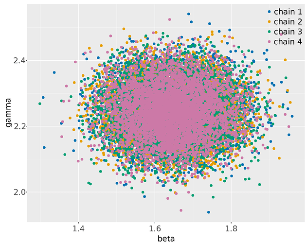
I’m not sure how to map chains to colors but here are the plots

jack_monroe · February 22, 2022, 10:53pm

That looks how I expected, how about trying it with a stronger prior on sigma? Maybe normal(0, 0.5) or normal(0.8, 0.2) or something that regularizes it toward (0.5,1) to a greater extent. Might not fix everything, but I think I’d start there.

abs · February 23, 2022, 9:14pm

Using the suggestions above does seem to fix the fit according to the diagnostics, but the answers don’t agree with the true parameters.

With

this generator

data {
  int<lower=0> N;
}
generated quantities {
  real x[N];
  real u[N];
  for (n in 1:N) {
    x[n] = normal_rng(0,1);
    u[n] = normal_rng(0,1);
  }
  real beta = normal_rng(1,1);
  real gamma = normal_rng(3,1);
  real<lower=0> sigma = uniform_rng(.5,1);
  real x_beta[N];
  real u_gamma[N];
  real mu[N];
  real y[N];
  for (n in 1:N) {
    x_beta[n] = x[n] * beta;
    u_gamma[n] = u[n] * gamma;
    mu[n] = x_beta[n] + u_gamma[n];
    y[n] = normal_rng(mu[n], sigma);
  }
}

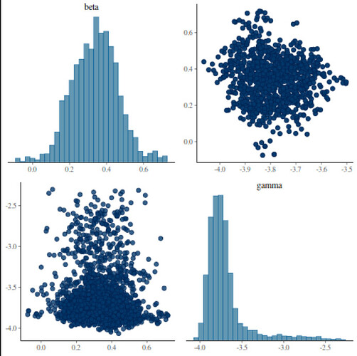
generating

{ "beta": 1.60753,  "gamma": 1.898,  "sigma": 0.779287 }

then sampling 5000 samples with

this model

data {
  int<lower=0> N;
  real y[N];
  real x[N];
}
parameters {
  real beta;
  real<lower=0> gamma;
  vector[N] u;
  real<lower=0> sigma;
}
model {
  real x_beta[N];
  real u_gamma[N];
  to_vector(u) ~ normal(0,1);
  beta ~ normal(0, 2);
  gamma ~ normal(3, .1);
  sigma ~ normal(1,.2);

  for (n in 1:N) {
    x_beta[n] = x[n] * beta;
    u_gamma[n] = u[n] * gamma;
    y[n] ~ normal(x_beta[n] + u_gamma[n], sigma);
  }
}

gives

Inference for Stan model: train_model
4 chains: each with iter=(5000,5000,5000,5000); warmup=(0,0,0,0); thin=(1,1,1,1); 20000 iterations saved.

Warmup took (4.8, 5.6, 5.7, 5.6) seconds, 22 seconds total
Sampling took (27, 36, 36, 36) seconds, 2.2 minutes total

                    Mean     MCSE  StdDev        5%       50%       95%    N_Eff  N_Eff/s    R_hat

lp__            -8.0e+01  2.8e+01     281  -4.9e+02  -1.1e+02   4.2e+02      102     0.76      1.1
accept_stat__       0.92  1.4e-03   0.094      0.72      0.95      1.00  4.6e+03  3.4e+01  1.0e+00
stepsize__         0.094  1.5e-02   0.021     0.082     0.082      0.13  2.0e+00  1.5e-02  1.4e+13
treedepth__          5.6  1.2e-01    0.50       5.0       6.0       6.0  1.7e+01  1.3e-01  1.2e+00
n_leapfrog__          50  3.8e+00      17        31        63        63  1.9e+01  1.4e-01  1.1e+00
divergent__         0.00      nan    0.00      0.00      0.00      0.00      nan      nan      nan
energy__             582  2.8e+01     282        85       614       998  1.0e+02  7.6e-01  1.1e+00

beta             1.6e+00  2.1e-03   0.068   1.5e+00   1.6e+00   1.8e+00     1026      7.6      1.0
gamma            2.2e+00  1.8e-03   0.054   2.2e+00   2.2e+00   2.3e+00      924      6.9      1.0
sigma            4.4e-01  1.1e-02    0.12   2.6e-01   4.4e-01   6.4e-01      107     0.79      1.0

which looks like

jack_monroe · February 23, 2022, 9:35pm

Which prior did you place on sigma? Maybe the Normal(0.8,0.2) would be better (if you used the Normal(0, 0.5)) because it doesn’t immediately diverge from the actual DPG.

abs · February 23, 2022, 10:27pm

The prior is given in the hidden “model” block in that post.

Now trying N(.8,.2)

data {
  int<lower=0> N;
  real y[N];
  real x[N];
}
parameters {
  real beta;
  real<lower=0> gamma;
  vector[N] u;
  real<lower=0> sigma;
}
model {
  real x_beta[N];
  real u_gamma[N];
  to_vector(u) ~ normal(0,1);
  beta ~ normal(0, 2);
  gamma ~ normal(3, .1);
  sigma ~ normal(.8,.2);

  for (n in 1:N) {
    x_beta[n] = x[n] * beta;
    u_gamma[n] = u[n] * gamma;
    y[n] ~ normal(x_beta[n] + u_gamma[n], sigma);
  }
}

when the true values are

{  "beta": 0.777222,  "gamma": 3.60909,  "sigma": 0.700439}

gives 90% CI that excludes the true value of sigma.

Inference for Stan model: train_model
4 chains: each with iter=(5000,5000,5000,5000); warmup=(0,0,0,0); thin=(1,1,1,1); 20000 iterations saved.

Warmup took (4.5, 5.0, 5.0, 5.4) seconds, 20 seconds total
Sampling took (19, 20, 20, 22) seconds, 1.4 minutes total

                    Mean     MCSE  StdDev        5%       50%       95%    N_Eff  N_Eff/s    R_hat

lp__            -1.2e+03  1.4e+01     187  -1.5e+03  -1.2e+03  -8.6e+02      171      2.1      1.0
accept_stat__       0.87  4.5e-03    0.13      0.60      0.91      1.00  8.5e+02  1.0e+01  1.0e+00
stepsize__          0.17  9.5e-03   0.013      0.14      0.17      0.18  2.0e+00  2.4e-02  4.8e+12
treedepth__          4.8  3.2e-02    0.41       4.0       5.0       5.0  1.6e+02  2.0e+00  1.1e+00
n_leapfrog__          28  5.0e-01     6.5        15        31        31  1.7e+02  2.0e+00  1.0e+00
divergent__         0.00      nan    0.00      0.00      0.00      0.00      nan      nan      nan
energy__            1707  1.4e+01     189      1356      1730      1970  1.7e+02  2.1e+00  1.0e+00

beta             7.6e-01  1.7e-03    0.11   5.9e-01   7.6e-01   9.3e-01     3682       45      1.0
gamma            3.3e+00  3.8e-03   0.080   3.1e+00   3.3e+00   3.4e+00      448      5.5      1.0
sigma            1.2e+00  1.5e-02    0.21   8.1e-01   1.2e+00   1.5e+00      195      2.4      1.0

jack_monroe · February 23, 2022, 10:59pm

You put a prior on gamma that restricts it to be wrong, maybe a wider prior?

abs · February 23, 2022, 11:10pm

Ah you’re right. This seems to work.

True:

{  "beta": 0.20741,  "gamma": 3.85316,  "sigma": 0.626882}

Model:

data {
  int<lower=0> N;
  real y[N];
  real x[N];
}
parameters {
  real beta;
  real<lower=0> gamma;
  vector[N] u;
  real<lower=0> sigma;
}
model {
  real x_beta[N];
  real u_gamma[N];
  to_vector(u) ~ normal(0,1);
  beta ~ normal(0, 2);
  gamma ~ normal(3, 1);
  sigma ~ normal(.8,.2);

  for (n in 1:N) {
    x_beta[n] = x[n] * beta;
    u_gamma[n] = u[n] * gamma;
    y[n] ~ normal(x_beta[n] + u_gamma[n], sigma);
  }
}

Results:

Inference for Stan model: train_model
4 chains: each with iter=(5000,5000,5000,5000); warmup=(0,0,0,0); thin=(1,1,1,1); 20000 iterations saved.

Warmup took (6.0, 4.6, 4.6, 4.6) seconds, 20 seconds total
Sampling took (31, 21, 21, 21) seconds, 1.6 minutes total

                    Mean     MCSE  StdDev        5%       50%       95%    N_Eff  N_Eff/s    R_hat

lp__            -7.2e+02  3.3e+01     298  -1.1e+03  -7.6e+02  -8.9e+01       84     0.88      1.1
accept_stat__       0.87  1.1e-02    0.15      0.55      0.92      1.00  2.1e+02  2.2e+00  1.0e+00
stepsize__          0.13  7.8e-03   0.011      0.11      0.13      0.13  2.0e+00  2.1e-02  5.2e+12
treedepth__          5.0  1.9e-01    0.52       4.0       5.0       6.0  7.8e+00  8.3e-02  1.2e+00
n_leapfrog__          34  5.3e+00      13        15        31        63  6.3e+00  6.7e-02  1.3e+00
divergent__         0.00      nan    0.00      0.00      0.00      0.00      nan      nan      nan
energy__            1222  3.3e+01     299       589      1264      1646  8.3e+01  8.8e-01  1.1e+00

beta             2.3e-01  3.7e-03    0.12   2.7e-02   2.3e-01   4.4e-01     1146       12      1.0
gamma            3.9e+00  4.3e-03   0.097   3.7e+00   3.9e+00   4.0e+00      511      5.4      1.0
sigma            7.9e-01  2.2e-02    0.21   4.0e-01   7.9e-01   1.1e+00       95      1.0      1.0

abs · February 25, 2022, 5:35am

I am looking at the document at 7.2 Change point models and Finite mixtures to understand marginalization.

I don’t understand how this rewrite works:
normal(x_beta[n] + u_gamma[n], sigma) to normal(x_beta[n], hypot(sigma, gamma)). Is there a simple demonstration, or perhaps another way of writing the marginalization that’s easier to see?

Can I interpret gamma the same way after marginalization?

nhuurre · February 25, 2022, 9:32am

Those discuss discrete parameters. Continuous parameters are the same in principle but use an integral instead of a sum

p\left(x\right)=\int_{-\infty}^\infty p\left(x,y\right)\mathrm{d}y

The original expression is equivalent to normal(x_beta[n], sigma) + gamma*normal(0,1) where I have moved and expanded u_gamma[n].

The sum of two normally distributed variables

X\sim\mathcal{N}\left(\mu_{x},\sigma_{x}\right) \\ Y\sim\mathcal{N}\left(\mu_{y},\sigma_{y}\right) \\ Z=X+Y

is also normally distributed

Z\sim\mathcal{N}\left(\mu_{x}+\mu_{y},\sqrt{\sigma_{x}^{2}+\sigma_{y}^{2}}\right)

Yes.

Topic		Replies	Views
Blog post: Identifying non-identifiability Publicity	11	4246	June 6, 2018
Weak identifiability in measurement models Modeling specification	3	498	January 20, 2020
Multiple modes in latent variable model -- identifiability, or something else? Modeling	0	437	May 16, 2018
Linear model where each x has it's own normal distribution Modeling	6	578	March 1, 2019
Help with misspecified model Modeling fitting-issues , specification	2	381	September 10, 2020

Fitting an unidentified linear model

Related Topics