Factor Mixture Modelling

Apologies in advance for the large model, I’ve tried to make it as reader-friendly as possible.

I’m attempting to estimate a mixture of latent factors using stan, and I wanted to make sure that my code was doing what I thought it was doing. The model has two parts: the measurement (factor) model, and the mixture model. The conceptual/statistical background is covered in this paper: http://www.statmodel.com/bmuthen/articles/Article_100.pdf

To make it more complicated, I’m also attempting to implement the BSEM approach of identification for cross-loadings and residual covariances (zero-mean, small variance priors), and relax the assumption of local independence (zero covariance within class) using the same approach. This is using ordinal data (33 items, 3 categories).

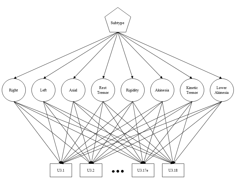
Here’s a diagram of what I’m aiming to estimate (circles represent latent variables and rectangles observed variables):

And here’s the model I’m using for it:

 data{
	int N;				//Observations
	int J;				//Items
	int E;				//Latent factors
	int K;				//Clusters
	int y[N,J];			//Responses
	int right[11];		//List of loadings
	int r_n[22];		//List of loadings
	int left[11];		//list of loadings
	int l_n[22];		//list of loadings
	vector[J] sig;		//sqrt((pi^2)/3) - SD of logistic residuals
	real i_var;			//sqrt(5) - SD of intended loadings/thresholds/cluster means
	real u_var;			//sqrt(0.01) - SD of cross-loadings
}

parameters{
	matrix[J,E] lam;					//Matrix of factor loadings
	row_vector[E] eta[N];				//Vector of factor scores
	vector[J] eps_raw[N];				//Vector of unobserved response variables: Non-centered parameterization
	ordered[(K-1)] mu_raw[E];			//Vector of latent factor means within cluster
	ordered[3] alpha[J];				//Item thresholds
	simplex[K] theta;					//Cluster proportions
	cholesky_factor_corr[E] e_Lcorr1;	//Latent factor correlations - Cluster 1
	cholesky_factor_corr[E] e_Lcorr2;	//Latent factor correlations - Cluster 2
	cholesky_factor_corr[E] e_Lcorr3;	//Latent factor correlations - Cluster 3
	cholesky_factor_corr[J] u_Lcorr;	//Residual covariances
}

transformed parameters{
	vector[J] epsilon[N];					//Unobserved response underlying categorical response
	vector[E] mu[K];						//Cluster means
	
	for(e in 1:E){							//Latent means are identified by fixing the means of the first cluster to 0
		mu[1,e] = 0;						//	and defining the means of the others by their difference from the first
		mu[2,e] = mu[1,e] - mu_raw[e,1];
		mu[3,e] = mu[1,e] - mu_raw[e,2];
			}
	
//Response is sum of loadings on Latents
	//Unobserved response response variable is MVN with mean equal to sum of loadings on
	//	each latent factor, i.e. (eta[n,1]*lam[j,1]) + ... + (eta[n,8]*lam[j,8]),
	//	SD of sqrt((pi^2)/3), and with correlations in u_Lcorr

	for(n in 1:N){
		epsilon[n] = (eta[n]*lam')' + (diag_pre_multiply(sig,u_Lcorr)*(eps_raw[n]));
				}
}
	
model{
	vector[K] contrib[N];				//Vector to hold log-probability contributions
	
//Factor Loadings
   //Right
	for(j in right[1]:right[11]){lam[j,1] ~ normal(0,i_var);}
	for(j in r_n[1]:r_n[22]){lam[j,1] ~ normal(0,u_var);}
			
   //Left
	for(j in left[1]:left[11]){lam[j,2] ~ normal(0,i_var);}
	for(j in l_n[1]:l_n[22]){lam[j,2] ~ normal(0,u_var);}
			
  //Axial
	lam[1,3]~ normal(0,i_var);
  	lam[2,3]~ normal(0,i_var);
  	lam[18,3]~ normal(0,i_var);
  	lam[19,3]~ normal(0,i_var);
  	lam[20,3]~ normal(0,i_var);
  	lam[21,3]~ normal(0,i_var);
  	lam[22,3]~ normal(0,i_var);
  	lam[23,3]~ normal(0,i_var);
	for(j in 3:17){lam[j,3]~ normal(0,u_var);}
	for(j in 24:33){lam[j,3]~ normal(0,u_var);}

   //Rest Tremor
	for(j in 28:33){lam[j,4]~ normal(0,i_var);}
	for(j in 1:27){lam[j,4]~ normal(0,u_var);}
	
   //Rigidity
	for(j in 3:7){lam[j,5]~ normal(0,i_var);}
	for(j in 1:2){lam[j,5]~ normal(0,u_var);}
	for(j in 8:33){lam[j,5]~ normal(0,u_var);}
	
   //Akinesia
	for(j in 8:13){lam[j,6]~ normal(0,i_var);}
	for(j in 1:7){lam[j,6]~ normal(0,u_var);}
	for(j in 14:33){lam[j,6]~ normal(0,u_var);}
		
   //Kinetic Tremor
	for(j in 24:27){lam[j,7]~ normal(0,i_var);}
	for(j in 1:23){lam[j,7]~ normal(0,u_var);}
	for(j in 28:33){lam[j,7]~ normal(0,u_var);}
		
   //Lower Akinesia
	for(j in 14:17){lam[j,8]~ normal(0,i_var);}
	for(j in 1:13){lam[j,8]~ normal(0,u_var);}
	for(j in 18:33){lam[j,8]~ normal(0,u_var);}
		
//Item Thresholds
	for(j in 1:J)
		for(r in 1:3)
			alpha[j,r] ~ normal(0,i_var);

//Latent Factor Means
	for(e in 1:E){
		mu_raw[e] ~ normal(0,i_var);
			}

//Within-cluster factor correlations
	e_Lcorr1 ~ lkj_corr_cholesky(50);
	e_Lcorr2 ~ lkj_corr_cholesky(50);
	e_Lcorr3 ~ lkj_corr_cholesky(50);

//Residual covariances
	u_Lcorr ~ lkj_corr_cholesky(50);
	
//Cluster proportions
	theta ~ dirichlet(rep_vector(10,K));

	for(n in 1:N){
	//Clustering process
		contrib[n,1] = log(theta[1]) + multi_normal_cholesky_lpdf(eta[n] | mu[1],e_Lcorr1);
		contrib[n,2] = log(theta[2]) + multi_normal_cholesky_lpdf(eta[n] | mu[2],e_Lcorr2);
		contrib[n,3] = log(theta[3]) + multi_normal_cholesky_lpdf(eta[n] | mu[3],e_Lcorr3);
		target += log_sum_exp(contrib[n,]);
	
	//'Raw' variable for non-centered unobserved response variable 
		eps_raw[n] ~ normal(0,1);
	
	//Observed data
		for(j in 1:J){y[n,j] ~ ordered_logistic(epsilon[n,j],alpha[j]);}
				}
 }// end of model
 
generated quantities{
	matrix[N,J] log_lik; 		//log-likeliood for psis-loo/waic
	vector[K] log_Pr[N];		//Individual log-probability of membership to each cluster

	for(n in 1:N){
		vector[K] prob;
		for(j in 1:J){
			log_lik[n,j] = ordered_logistic_lpmf(y[n,j] | epsilon[n,j],alpha[j]);
				}
		prob[1] = log(theta[1]) + multi_normal_cholesky_lpdf(eta[n] | mu[1],e_Lcorr1);
		prob[2] = log(theta[2]) + multi_normal_cholesky_lpdf(eta[n] | mu[2],e_Lcorr2);
		prob[3] = log(theta[3]) + multi_normal_cholesky_lpdf(eta[n] | mu[3],e_Lcorr3);
		
		log_Pr[n,1] = prob[1] - log_sum_exp(prob);
		log_Pr[n,2] = prob[2] - log_sum_exp(prob);
		log_Pr[n,3] = prob[3] - log_sum_exp(prob);
			}

}

First of all, is this estimating the model that I’m trying to estimate? And secondly, are there any ways of optimising this? I’ve tried to vectorise and use the non-centered parameterization where possible, but any suggestions would be greatly appreciated.

Let me know if I can provide any more info to help clarify, I’d be very grateful for any help.

Cheers,
Andrew

Hi Andrew,

Your questions are really broad and we’re trying to publish answers to those in more permanent form. Two things would be helpful from you:

  • to really be confident you are estimating the model you want to estimate you (or I, or anyone else) would need to code a simulation for it, and see if the parameters you estimate match what you used to generate your data. If you do that and you can’t figure out why they don’t match up you’ve reduced your really broad question to a specific one somebody here will have time to answer

  • To optimize your model it’s helpful to first know you 1) have the model you want (above); and 2) know that it is converging. I wouldn’t worry about it before that. For efficiency you are already using LKJ priors and the matching normal_*_lpdf so to a first order it’s optimized. The normal density is defined for vectors (and it is more efficient to use it that way) so all the places you have loops so you can do scalar ~ N(0,var) you can avoid looping and just do vector ~ N(0,var), except that our normal is prameterized w/standard deviation not variance, so it’s vector ~ normal(0,sd).

Hope that helps. You will tend to get more complete answers here if you can narrow down your problem and of course once you know you have what you want and it’s converging it’s always fun to make it go faster.

I sound like a broken record on our forums, but before jumping to this huge model, take a simple subset of it, code it in Stan, simulate data for it, and make sure it fits. Then once you know the technique works, build it out. It’s madness trying to debug something with this much cut-and-paste code.

One thing you’re going to want to do is pull some of this out into functions to remove code duplication.

For efficiency, you want to vectorize. But mixtures of multivariate normals may be problematic. Michael wrote a case study on mixture models, and things are only harder in multiple dimensions (see the web site under case studies under the docs tab).

I’ve never seena nyone try an lkj_corr_cholesky(50)—you wanted lots of prior mass around the unit correlation matrix? (I realize I don’t have any intuition for how strong the pull is).

The main thing you want to do for efficiency is vectorize, but the computation’s all going to be dominated here by the multivariate normals. See the manual chapter on optimizing/efficiency. You can also use slicing. So where you write

for(j in 14:17){lam[j,8]~ normal(0,i_var);}

you can just have

lam[14:17, 8] ~ normal(0, i_var);

Easier to read and faster.

Is there no way to group any of those variables or describe them with data that doesn’t involve all this hard-coding of indexes?

Hi Sakrejda and Bob,

Thanks for your responses. You’re right, I should have been much clearer about my process and what I was asking. Hopefully this clears things up.

In terms of simulation and appropriateness of the model, I’m already reasonably confident. The aim of the code is to replicate a model that I’ve already run in a different program (Mplus). I did take a stepwise approach to building the model, moving from ordinal regression, to a one-factor model, two-factor model with cross-loadings, etc., comparing the results to an equivalent model run in Mplus at each stage.

The magnitude, sign (positive/negative), and substantive interpretation of the parameters are generally consistent between models. I can’t directly compare the values of parameters, as Mplus only has the ordered probit model with Bayes and Stan only has the ordered logit.

I’m less concerned about the ‘correctness’ of the model, since it runs, converges, and is broadly consistent with the model I’m trying to replicate. I was more asking if I’d made any large-scale errors with the coding (i.e. type declarations, order of sampling statements, etc.). My Bayesian experience is limited to JAGS and Mplus, both of which have fairly different coding conventions to stan.

The LKJ prior is being used for model identification. With a factor model you can’t estimate all residual covariances between observed items, as there will not be enough restrictions for the model to be identified. The proposal is to use a strong prior that the residual covariances should be 0. This should set the residual covariances to approximately zero, allowing for identification, while also allowing the estimated parameter to be greater than this if the relationship in the observed data is strong enough. The background for this is here: https://www.statmodel.com/download/BSEMv4REVISED

Based on these simulations an LKJ prior with eta=50 looks to approximate a strong prior that the resulting correlation should be 0. But I still need to do some sensitivity analyses and look at different specifications.

For the optimization, that slicing for the ‘lams’ will be quite useful. Is there a way of using this with a non-sequential list of numbers? For example, changing:

	lam[1,3]~ normal(0,i_var);
  	lam[2,3]~ normal(0,i_var);
  	lam[18,3]~ normal(0,i_var);
  	lam[19,3]~ normal(0,i_var);
  	lam[20,3]~ normal(0,i_var);
  	lam[21,3]~ normal(0,i_var);
  	lam[22,3]~ normal(0,i_var);
  	lam[23,3]~ normal(0,i_var);

to something like:

lam[c(1,2,18:23),3]~ normal(0,i_var);

I hadn’t considered different ways of passing the factor loading specifications. That could be very helpful in generalising this in the future, I’ll have a look into that.

For the computational burden of the multivariate normals, is there a way of coding this with the non-centered parameterization from the manual, while still recording the correct log-probability contributions for each cluster?

Apologies again for not being more clear in the first post, and for the size of this one!

Thanks,
Andrew

We don’t have that general syntax for using 18:23 to construct a 6-element array. The closest you could get would be

append(lam[{1, 2}], lam[18:23]) ~ normal(0, i_var)

or

lam[{1, 2, 18, 19, 20, 21, 22, 23}, 3] ~ normal(0, i_var);

It would be even more efficient if you construct these indexing arrays in transformed data (where they only need be computed once).

transformed data {
  int idxs[8] = {1, 2, 18, 19, 20, 21, 22, 23};
...
model {
  lam[idxs, 3] ~ normal(0, i_var);

Stan uses scale, not variance for normals (in case the var in i_var was supposed to mean variance).

This can all be vectorized:

for (e in 1:E) {
mu[1, e] = 0;
mu[2, e] = mu[1, e] - mu_raw[e, 1];
mu[3, e] = mu[1, e] - mu_raw[e, 2];
}

as

mu[1] = rep_vector(0, E);
mu[2] = mu[1] - mu_raw[ , 1];
mu[3] = mu[1] - mu_raw[ , 2];

It won't be any faster as there are no shared computations, but it's shorter and easier to read.  You could move the definition of that `rep_vector(0, E)` to transformed data, too so it doesn't need to be continually created.

The main thing to do is avoid recomputation.  You should read the optimization chapter of the manual at this point.  For example, in this

for (n in 1:N){
epsilon[n] = (eta[n]lam’)’ + (diag_pre_multiply(sig,u_Lcorr)(eps_raw[n]));


you could use matrix arithmetic to compute `eta * lam` once, but you'd need to make sure that eta was defined as a matrix.  Matrix multiply is much faster than doing what you're doing here (it is good to use what you used for `eta` to index bu tnot to multiply.  But the really huge savings will be from taking the diagonal pre-multiply and designing it on the top.  You should also rearrange data types so you don't need to do all that transposition.  You should be able to write this in the form

epsion = eta * lam + diag_pre_multiply(sig, u_Lcorr) * eps_raw;


and it'll be a lot faster.  (We really need a `diag_pre_multiply_tri` version if we know the second argument is lower triangular.)

Anyway, I'll let you try to work through other optimizations after reading the manual chapter.

Hi Bob,

Those suggestions sound great, I’ll work through those and the manual chapter.

Thanks (to you and the other developers) for all your work with Stan and these forums, much appreciated.

Andrew