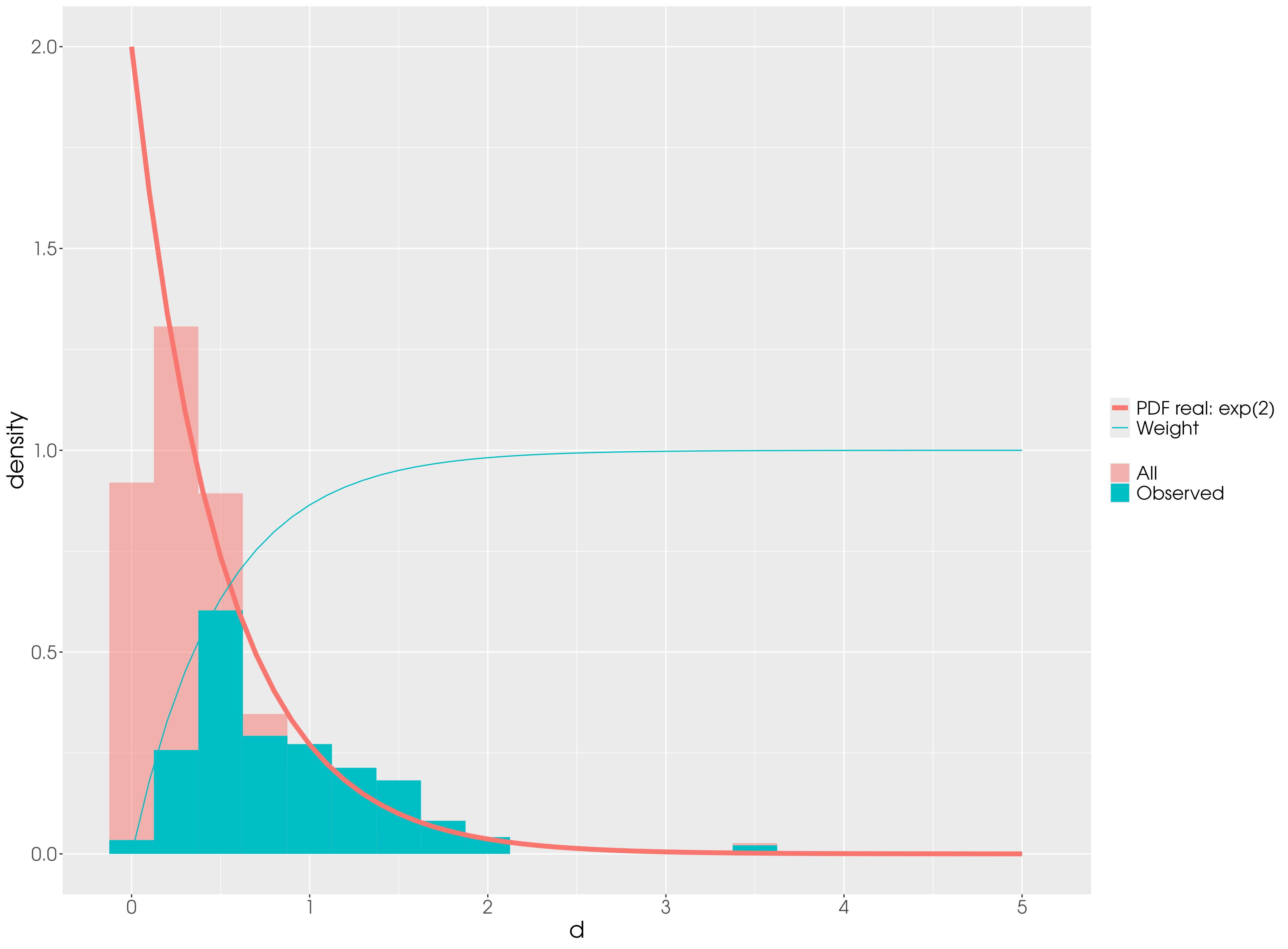
Estimate distribution with missing values and weight function

GianniRewer · February 23, 2024, 3:27pm

I would like to estimate the parameter of a distribution but there are some data missing (let’s say about 50%). The data are not missing at random, however, but they are dependent on a weighting function. Basically, we can trust the tail of the distribution, but not the bulk of it. In the figure below, the red distribution is the complete data but we observed only the blue one. Our hypothesis is that the observed data were sampled from the complete distribution according to a weighting function (in this specific case it is the cumulative distribution function of the exponential distribution)

My attempt was to attach a weight to each observed data point and run

m <- brm(d|weights(w) ~ 1,
    family = exponential,
    ...
)

but this has not yielded a good fit. The real lambda is 2 but the estimate is about 0.84 as shown by the black lines in the figure below:

Do you have any suggestions on how I could incorporate a “weighting/missingness” function in the model? Ideally, I would also want to estimate the parameters of that function.

I attach a minimal working example that generates the data, fit, and figures:

library("tidyverse")
library("brms")
library("tidybayes")

SEED <- 20220510
set.seed(SEED)

RATE  <- 2
N  <- 300
X  <- seq(0, 5, by=0.1)
P_BIAS  <- 0.5
exp_pdf  <- tibble(
    x = X,
    pdf = dexp(x, rate = RATE))

w_curve  <- tibble(x = X, y = pexp(x, rate = RATE))

df <- tibble(d = rexp(N, rate = RATE), w = pexp(d, rate = RATE))
df_biased  <- df  %>% sample_frac(size = P_BIAS, replace = TRUE, weight = w)  %>%
    mutate(w_post =  pexp(d, rate = RATE))

df %>%
    ggplot() +
    geom_histogram(aes(x = d, y=after_stat(density), fill = 'All'), alpha = 0.5, position = "identity",binwidth = 0.25) +
    geom_histogram(aes(x = d, y=after_stat(density)*P_BIAS, weight=w, fill = 'Observed'), position = "identity",binwidth = 0.25, data = df_biased) +
    geom_line(aes(x=x, y=pdf, color=sprintf('PDF real: exp(%d)', {{RATE}})), size=2, data=exp_pdf) +
    geom_line(aes(x=x, y=y, color = 'Weight'), data=w_curve) + 
    labs(color = NULL, fill = NULL) + 
    theme(text = element_text(size=20))


ggsave('empirical.png')

m <- brm(d|weights(w) ~ 1,
    data = df_biased,
    family = exponential,
    seed = SEED,
    file = 'exponential-bias.rds'
)

fit <- tibble(remove =NA) %>%
    tidybayes::add_epred_draws(m, transform = T, seed = SEED)  %>%
    ungroup()  %>%
    select(-c(.chain, .iteration, remove)) %>%
    mutate(x = list(X))  %>%
    rowwise()  %>%
    mutate(
        lambda = 1/.epred,
        pdf=list(dexp(x, rate=lambda))
    )  %>%
    unnest(cols = c(x, pdf))

fit_sample  <- fit  %>%
    sample_draws(25, seed = SEED)

df %>%
    ggplot() +
    geom_histogram(aes(x = d, y=after_stat(density), fill = 'All'), alpha = 0.5, position = "identity",binwidth = 0.25) +
    geom_histogram(aes(x = d, y=after_stat(density)*P_BIAS, weight=w, fill = 'Observed'), position = "identity",binwidth = 0.25, data = df_biased) +
    geom_line(aes(x=x, y=pdf, color=sprintf('PDF real: exp(%d)', {{RATE}})), size = 2, data=exp_pdf) +
    geom_line(aes(x=x, y=y, color = 'Weight'), data=w_curve) + 
    geom_line(aes(x=x, y=pdf, group=.draw),alpha = 0.25, data=fit_sample) +
    labs(color = NULL, fill = NULL) +
    theme(text = element_text(size=20))


ggsave('fit.png')

jsocolar · February 23, 2024, 3:55pm

What parametric assumptions do you want to make about

The underlying distribution?
What you call the weighting function, giving the probability that an observation is not missing, conditional on the value of that observation?

Once you define these, your model is that the data are sampled from the normalized product of the PDF from (1) and the function from (2). So depending on the functional forms desired, let’s see if we can work out a closed-form expression for what that normalizing constant should be, which would allow you to define a custom brms family that fits your data efficiently.

GianniRewer · February 23, 2024, 9:44pm

I am pretty confident the underlying distribution is an exponential one

I am not sure I fully understand this, sorry. The probability of the observations is conditional on the weighting function (I am sure there is a better name for it!). Also here, I am pretty sure this probability is close to zero as we approach zero, and close to one as we tend to infinity (The tail of the distribution of the observations would closely match the one of the underlying distribution). As I used in the example, it is reasonable that the probability of observing a data point is the CDF of an exponential. Perhaps by having two equations related to an exponential distribution makes it convenient to find a close form solution?

In the end, I want to find the parameter lambda of the underlying exponential distribution.

Does it make sense?

jsocolar · February 23, 2024, 10:18pm

By assumption, the true underlying distribution has probability density function \lambda e^{-\lambda x}. The observed data are distributed according to something proportional to \lambda e^{-\lambda x} * (1 - e^{-mx}) (the second term being the exponential CDF, again by assumption). To turn this into a probability density function over x, we need to divide by a normalizing constant equal to \int_0^\infty \lambda e^{-\lambda x} * (1 - e^{-mx})dx. Distributing the product and separating the terms we have 1 - \int_0^\infty \lambda e^{-(m + \lambda)x}dx, which simplifies to \frac{m}{m+\lambda}.

Thus, the log probability density function from which you need to sample is given by \log(\frac{m+\lambda}{m} \lambda e^{-\lambda x} * (1 - e^{-mx})). This is a two parameter distribution parameterized by m and \lambda. If desired, you can implement this as a custom family in brms following the vignette here Define Custom Response Distributions with brms.

GianniRewer · February 24, 2024, 5:19pm

oh wow, this is excellent and looks super promising. I am gonna try and report back.

GianniRewer · February 26, 2024, 9:53am

Ok @jsocolar, I think my attempt based on your help was successful.

I implemented your log PDF as a Stan function and created a custom family in brms:

stan_funs <- "
  real exponential_bias_lpdf(real y, real mu, real m) {
    return log((m + mu)/m * mu * exp(-mu * y) * (1 - exp(-m*y)));
  }
"

stanvars <- stanvar(scode = stan_funs, block = "functions")

m2 <- brm(bf(d ~ 1),
    data = df_biased,
    family = exponential_bias,
    stanvars = stanvars,
    seed = SEED,
    prior = prior_string("normal(0,5)", class = "m", lb = 0),
    file = 'exponential-bias-2.rds',
    file_refit = "on_change"
)

yielded:

 Family: exponential_bias 
  Links: mu = log; m = identity 
Formula: d ~ 1 
   Data: df_biased (Number of observations: 150) 
  Draws: 4 chains, each with iter = 2000; warmup = 1000; thin = 1;
         total post-warmup draws = 4000

Population-Level Effects: 
          Estimate Est.Error l-95% CI u-95% CI Rhat Bulk_ESS Tail_ESS
Intercept     0.75      0.15     0.50     1.07 1.00      946     1070

Family Specific Parameters: 
  Estimate Est.Error l-95% CI u-95% CI Rhat Bulk_ESS Tail_ESS
m     3.50      2.04     0.26     8.00 1.00      942      918

Draws were sampled using sampling(NUTS). For each parameter, Bulk_ESS
and Tail_ESS are effective sample size measures, and Rhat is the potential
scale reduction factor on split chains (at convergence, Rhat = 1).

The lambda parameter (called mu in brms) is not too far from 2 (exp(0.75) = 2.117). The sampling is also fine. The m parameter seems to be much harder to sample precisely (it should be too around 2 but at least it is within the uncertainty interval).

Do you know how I could get a higher precision in the m parameter estimate? What I am thinking is that I sort of expect the observed values to be a x% of the total (unobserved) distribution. In this case, I simulated the data assuming there is a bias of 50%. Do you know how I could add also this prior info?

I wonder if it would help to optimized the Stan function I wrote (e.g., I changed 1 - exp(-m*y) to -expm1(-m*y) but nothing major changed).

Bonus attempt

I also tried to reuse Stan functions to create a custom distribution in brms:

stan_funs <- "
  real exponential_bias_lpdf(real y, real mu, real m) {
    return exponential_lpdf(y | mu) * exponential_cdf(y, m);
  }
"

but the sampling was horrible. I thought it would work :)

EDIT: I also realized an error in my previous post:

fit <- tibble(remove =NA) %>%
    tidybayes::add_epred_draws(m, transform = T, seed = SEED)  %>%
    ungroup()  %>%
    select(-c(.chain, .iteration, remove)) %>%
    mutate(x = list(X))  %>%
    rowwise()  %>%
    mutate(
        lambda = 1/.epred,
        pdf=list(dexp(x, rate=lambda))
    )  %>%
    unnest(cols = c(x, pdf))

should be

fit <- tibble(remove =NA) %>%
    tidybayes::add_epred_draws(m, transform = T, seed = SEED)  %>%
    ungroup()  %>%
    select(-c(.chain, .iteration, remove)) %>%
    mutate(x = list(X))  %>%
    rowwise()  %>%
    mutate(
        lambda = .epred,
        pdf=list(dexp(x, rate=lambda))
    )  %>%
    unnest(cols = c(x, pdf))

where now lambda = .epred. I got confused as Stan uses the reciprocal of the rate parameter.

jsocolar · February 26, 2024, 12:14pm

The fraction of the values expected to be observed (not the fraction actually realized in the sample; the expectation) is \frac{m}{m+\lambda}. You can add a prior on this, but you should carefully check that actual prior distribution that this induces on m and \lambda as this quantity is nonlinear in those terms.

GianniRewer:

I also tried to reuse Stan functions to create a custom distribution in brms:
stan_funs <- "
  real exponential_bias_lpdf(real y, real mu, real m) {
    return exponential_lpdf(y | mu) * exponential_cdf(y, m);
  }
"
but the sampling was horrible. I thought it would work :)

There are two problems here. The first is that on the log scale things don’t multiply; they add. The second is that you are missing the normalizing term, which is not constant in the parameters and so cannot be dropped. If you want, you could instead return:

log(m+lambda) - log(m) + exponential_lpdf(y | mu) + exponential_lcdf(y, m);

I haven’t tested for correctness, but that should work I think.

GianniRewer · February 26, 2024, 12:36pm

jsocolar:

There are two problems here. The first is that on the log scale things don’t multiply; they add. The second is that you are missing the normalizing term, which is not constant in the parameters and so cannot be dropped. If you want, you could instead return:
log(m+lambda) - log(m) + exponential_lpdf(y | mu) + exponential_lcdf(y, m);
I haven’t tested for correctness, but that should work I think.

Of course they add (facepalm)! And I thought you could drop the normalizing constant. Thank you for explaining why it cannot.

The formula was almost right :)

stan_funs <- "
  real exponential_bias_lpdf(real y, real mu, real m) {
    return log(m+mu) - log(m) + exponential_lpdf(y | mu) + exponential_lcdf(y | m);
  }
"

I tried and it seems to be the same as the one you suggested in earlier post (but sampling feels much faster).

I am playing around with different values for the rates now. Sometimes it is quite hard to estimate them. Let me experiment a bit more and I’ll get back to you. Thank you again!

Topic		Replies	Views
Sample from parameterized distribution rather than estimate parameter brms	22	1006	March 23, 2023
How to update a brmsfit object with a modified brms-generated stan model marginalizing over a distribution of weights Modeling techniques , specification	9	2770	December 20, 2021
Survey weights in brms/stan - Simulation based on design effect, feedback sought! Modeling techniques	12	2525	September 9, 2022
Weights in brm brms	12	10850	February 21, 2022
Error with custom family Modeling brms	11	661	December 10, 2023

Estimate distribution with missing values and weight function

Bonus attempt

Related topics