Efficient rewriting of the 4 parameter logistic -- log1p_exp gives WORSE performance

I have been trying to write a scaled logistic model using Stan’s composed functions.
I thought this would be good for two reasons:

  1. I want to work on the log scale. The model I’m writing will be built out into something more complicated later and that would be convenient
  2. I thought that the greater efficiency of composed functions would make sampling better and more effective

however I’m surprised to find that writing things out “directly” gives better results! I’d like to know if this surprises anyone else, or if there is another reason for these observations

the model

I’m using the commonplace “4 parameter” or scaled logistic function:

Y = \left( L + \frac{U - L}{1 + e^{-\alpha \times (x)}} \right)

Note that for right now I’m leaving off the intercept, -\alpha(x - \beta)

I fit a minimal version of this model. I’m using poisson_log because I want to work on the log scale, which is a closer analogy to the usecase.

data {
  int<lower=0> N;
  vector[N] x_vals;
  array[N] int y_count;
}
parameters {
  real m;
  real u;
  real log_alpha;
}
model {
  m ~ normal(.69, .1);
  u ~ normal(2.3, .1);
  log_alpha ~ normal(0, .1);
  vector[N] log_mu;
  
  profile("meanpart"){
      log_mu = log(exp(m) + (exp(u) - exp(m)) ./ (1 + exp(-exp(log_alpha) * (x_vals))));;
  }

  y_count ~ poisson_log(log_mu);
}

The part I’m talking about is indicated by the profile statement.

I thought there was no way that it is efficient to be exponentiating and then taking the log of the expression – better to work directly on the log scale, right?

Here are different ways I’ve tried to write this part. They are in descending order of “success”, measured as time for the profile part and also ESS:

  1. log_mu = log(exp(m) + (exp(u) - exp(m)) * inv_logit(exp(log_alpha) * x_vals));
  2. log_mu = log(exp(m) + (exp(u) - exp(m)) ./ (1 + exp(-exp(log_alpha) * (x_vals))));
  3. log_mu = m + log1p(exp(f) * inv_logit(exp(log_alpha) * x_vals));
  4. log_mu = m + log1p_exp(f - log1p_exp(-exp(log_alpha) * x_vals));
  5. log_mu = m + log1p_exp(f + log_inv_logit(exp(log_alpha) * x_vals));

In the last three, I’m rewriting the expression using the same logic as the log_sum_exp trick (see below). I thought it would be helpful to have a parameter f = \ln((U-L)/L)

\begin{align} Y &= \left( L + \frac{U - L}{1 + e^{-\alpha(x - \beta)}} \right) \\ &= \left( L + \frac{L(1 + e^f) - L}{1 + e^{-\alpha(x - \beta)}} \right) \\ &= L\left( 1 + \frac{1 + e^f - 1}{1 + e^{-\alpha(x - \beta)}} \right) \\ &= L\left(1 + \frac{e^f}{1 +e^{-\alpha(x - \beta)}}\right) \\ \ln(Y) &= \ln\left(L\left(1 + \frac{e^f}{1 +e^{-\alpha(x - \beta)}}\right)\right) \\ &=\ln(L) + \ln\left(1 + \frac{e^f}{1 +e^{-\alpha(x - \beta)}}\right) \\ &=\ln(L) + \ln(1 + \frac{e^f}{1 +e^{-\alpha(x - \beta)}}) \\ &=\ln(L) + \ln(1 + e^{f + \text{log_inv_logit}(\alpha(x - \beta))}) \\ &=\ln(L) + \text{log1p_exp}(f + \text{log_inv_logit}(\alpha(x - \beta))) \\ &= m + \text{log1p_exp}(f - \text{log1p_exp}(-\alpha(x - \beta))) \end{align}

options 1 & 2 profile at about half the time as 3,4 and 5, and with double the ESS. I’m surprised and a little dismayed, since I thought refactoring the equation would improve performance.

What do you think? are my problems due to something else perhaps?

2 Likes

How does this work for you?

data {
  int<lower=0> N;
  vector[N] x_vals;
  array[N] int y_count;
}
parameters {
  real m;
  real u;
  real log_alpha;
}
model {
  m ~ normal(.69, .1);
  u ~ normal(2.3, .1);
  log_alpha ~ normal(0, .1);
  vector[N] log_mu;
  
  profile("meanpart"){
      // log_mu = log(exp(m) + (exp(u) - exp(m)) ./ (1 + exp(-exp(log_alpha) * (x_vals))));
       vector[N] log_mu_m_l = log_inv_logit(exp(log_alpha) * x_vals) + log(u - m);
       log_mu = log(exp(log_mu_m_l) - m);
  }

  y_count ~ poisson_log(log_mu);
}

This is the R code I used to simulate

library(rethinking)
library(cmdstanr)

N <- 100
x <- rnorm(N)
L <- rnorm(1, .69, .1)
U <- rnorm(1, 2.3, .1)
log_alpha <- rnorm(1)
alpha <- exp(log_alpha)

mu = L + (U - L) / inv_logit(alpha * x)

y <-vector()
for (i in 1:N)
  y[i] <- rpois(1, mu[i])

mod <- cmdstan_model("model.stan")

mod_user <- mod$sample(
  data = list(
    N = N,
    x_vals = x,
    y_count = y
  ),
  parallel_chains = 4
)
1 Like

There’s an error in your derivation starting on function 3. If I expose your functions and test

functions {
  real f1 (real m, real u, real log_alpha, real x) {
    return log(exp(m) + (exp(u) - exp(m)) * inv_logit(exp(log_alpha) * x));
  }
  
    real f2 (real m, real u, real log_alpha, real x) {
    return log(exp(m) + (exp(u) - exp(m)) ./ (1 + exp(-exp(log_alpha) * (x))));
  }
  
    real f3 (real m, real u, real log_alpha, real x) {
     real f = log( (u - exp(m)) / exp(m) );
      
    return m + log1p(exp(f) * inv_logit(exp(log_alpha) * x));
  }
  
    real f4 (real m, real u, real log_alpha, real x) {
      real f = log( (u - exp(m)) / exp(m) );
    return m + log1p_exp(f - log1p_exp(-exp(log_alpha) * x));
  }
  
    real f5 (real m, real u, real log_alpha, real x) {
      real f = log( (u - exp(m)) / exp(m) );
    return m + log1p_exp(f + log_inv_logit(exp(log_alpha) * x));
  }
}

I get

L <- 0.5567503
u <- 2.359621
log_alpha <- -1.304145
x <- -0.006315413
 
> f1(m = log(L), u = U, log_alpha = log_alpha, x = x)
[1] 1.716955
> f2(m = log(L), u = U, log_alpha = log_alpha, x = x)
[1] 1.716955
> f3(m = log(L), u = U, log_alpha = log_alpha, x = x)
[1] 0.3766632
> f4(m = log(L), u = U, log_alpha = log_alpha, x = x)
[1] 0.3766632
> f5(m = log(L), u = U, log_alpha = log_alpha, x = x)
[1] 0.3766632

Hi @spinkney , thank you so much for thinking about this!

If we model both L and U using exponentials, then your functions f3, f4 and f5 should be

real f = log( (exp(u) - exp(m)) / exp(m) )

If I edit your example with that change I get the same answer for all 5 functions

1 Like

Edit: fixed the issue

When you add in f

f = log( (exp(u) - exp(m)) / exp(m) );

we have to make sure that u > m or things fail due to \log(x) \le 0 by declaring a lower bound of m on u:

functions {
  vector f1 (real m, real u, real log_alpha, vector x) {
    return log(exp(m) + (exp(u) - exp(m)) * inv_logit(exp(log_alpha) * x));
  }
  
    vector f2 (real m, real u, real log_alpha, vector x) {
    return log(exp(m) + (exp(u) - exp(m)) ./ (1 + exp(-exp(log_alpha) * (x))));
  }
  
    vector f3 (real m, real u, real log_alpha, vector x) {
     real f = log( (exp(u) - exp(m)) / exp(m) );
      
    return m + log1p(exp(f) * inv_logit(exp(log_alpha) * x));
  }
  
    vector f4 (real m, real u, real log_alpha, vector x) {
      real f = log( (exp(u) - exp(m)) / exp(m) );
    return m + log1p_exp(f - log1p_exp(-exp(log_alpha) * x));
  }
  
    vector f5 (real m, real u, real log_alpha, vector x) {
      real f = log( (exp(u) - exp(m)) / exp(m) );
    return m + log1p_exp(f + log_inv_logit(exp(log_alpha) * x));
  }
  
   vector f6 (real m, real u, real log_alpha, vector x) {
      real a = log_diff_exp(u, m);
      return log(exp(log_inv_logit(exp(log_alpha) * x) + a) + exp(m));
   }
}
data {
  int<lower=0> N;
  vector[N] x_vals;
  array[N] int y_count;
  int test;
}
parameters {
  real m;
  real<lower=m> u;
  real log_alpha;
}
model {
  m ~ normal(.69, .1);
  u ~ normal(2.3, .1);
  log_alpha ~ normal(0, .1);
  vector[N] log_mu;
  
  profile("meanpart"){
    if (test == 1) log_mu = f1(m, u, log_alpha, x_vals); 
    if (test == 2) log_mu = f2(m, u, log_alpha, x_vals); 
    if (test == 3) log_mu = f3(m, u, log_alpha, x_vals); 
    if (test == 4) log_mu = f4(m, u, log_alpha, x_vals);   
    if (test == 5) log_mu = f5(m, u, log_alpha, x_vals); 
    if (test == 6) log_mu = f6(m, u, log_alpha, x_vals); 
  }

  y_count ~ poisson_log(log_mu);
}

I dialed up N to 500 and set init = 0. The profile I’m getting (restricted to chain 1)

      name   thread_id total_time forward_time reverse_time chain_stack no_chain_stack autodiff_calls no_autodiff_calls
1 meanpart 0x1023fc580    1.51117     1.042620     0.468550    85878576      127880697          85192                 1
2 meanpart 0x102df8580    1.56843     1.063630     0.504792   127023093      126349677          84172                 1
3 meanpart 0x1028d4580    1.41384     0.980008     0.433833    78730614      116888874          77869                 1
4 meanpart 0x1052d0580    2.22812     1.782170     0.445948    79277565      117700915          78410                 1
5 meanpart 0x100b10580    2.23300     1.615400     0.617599    81598910      121267291          80786                 1
6 meanpart 0x100e94580    2.03609     1.365280     0.670809   119877600      119479600          79600                 1

and the summary

     function_num  variable         mean       median         sd        mad            q5          q95     rhat  ess_bulk  ess_tail
 1:            1      lp__ 12070.801425 12071.100000 1.29034558 1.03782000 12068.3000000 12072.200000 1.005191 1180.2982 1354.3758
 2:            1         m     1.195003     1.188090 0.15630067 0.16003926     0.9484264     1.458634 1.004383  864.5290  918.8908
 3:            1         u     3.235323     3.237425 0.02596496 0.02485579     3.1897360     3.273461 1.003638 1082.2300 1253.5070
 4:            1 log_alpha    -1.172321    -1.173555 0.06761875 0.06604242    -1.2797665    -1.060348 1.003441 1133.0891 1270.4131
 5:            2      lp__ 12070.843600 12071.200000 1.30360419 1.03782000 12068.3000000 12072.200000 1.004099 1254.1928 1273.5621
 6:            2         m     1.182296     1.176225 0.15538083 0.15373079     0.9390752     1.444116 1.003086  941.0985  851.2797
 7:            2         u     3.237072     3.238710 0.02559389 0.02411449     3.1924940     3.275494 1.002523 1129.9751 1052.8702
 8:            2 log_alpha    -1.176101    -1.178710 0.06761722 0.06686526    -1.2863335    -1.065909 1.007272  973.6478 1011.7441
 9:            3      lp__ 12070.850025 12071.200000 1.28712827 1.03782000 12068.3000000 12072.200000 1.006723  915.8393 1300.5246
10:            3         m     1.183009     1.176940 0.15430859 0.14833413     0.9398430     1.456386 1.006221  743.4855  684.3262
11:            3         u     3.236955     3.239535 0.02609720 0.02398847     3.1883895     3.275487 1.003496  917.7627  876.7193
12:            3 log_alpha    -1.181286    -1.184330 0.06608252 0.06323289    -1.2847465    -1.068065 1.004086  889.8082  898.7382
13:            4      lp__ 12070.895500 12071.300000 1.28058374 1.03782000 12068.4000000 12072.200000 1.001190 1227.4695 1153.5177
14:            4         m     1.182510     1.172360 0.14945022 0.14613247     0.9547813     1.434469 1.002609  991.2870  963.5060
15:            4         u     3.237414     3.239330 0.02574801 0.02383280     3.1921755     3.274864 1.001454 1205.7290 1071.9978
16:            4 log_alpha    -1.175862    -1.179625 0.06590677 0.06532336    -1.2803280    -1.065165 1.002711 1058.4495 1320.4050
17:            5      lp__ 12070.964250 12071.300000 1.18761085 0.88956000 12068.7000000 12072.200000 1.001223 1360.0919 1466.1354
18:            5         m     1.181740     1.177110 0.14329230 0.13803006     0.9562818     1.420108 1.004639  769.2626 1092.0469
19:            5         u     3.237701     3.238920 0.02394965 0.02203885     3.1982090     3.274411 1.002662 1080.4420 1317.4606
20:            5 log_alpha    -1.178822    -1.180625 0.06612702 0.06512320    -1.2844205    -1.068883 1.001055 1038.0914 1013.3272
21:            6      lp__ 12070.886700 12071.200000 1.32131926 1.03782000 12068.3950000 12072.200000 1.003591 1289.0510 1128.9090
22:            6         m     1.183151     1.173420 0.15385343 0.13785956     0.9468537     1.436916 1.003629  879.4904  746.0398
23:            6         u     3.237005     3.239880 0.02720110 0.02332871     3.1940190     3.274209 1.002197 1096.4475  953.4095
24:            6 log_alpha    -1.176532    -1.178840 0.06909790 0.06626481    -1.2823950    -1.069609 1.002519  994.8720 1097.3767

thanks @spinkney ! here is a plot of the results of your tests (with the minor bug in the function names corrected! )

function_compare <- cmdstanr::cmdstan_model("spinkney_test.stan")

m <- rnorm(1, log(2), sd = .1)
f <- rnorm(1, log(10), sd = .1)
a <- rnorm(1, 0, .1)
b <- 0
x_vals <- runif(50, -6, 12)
y_mean <- m + log1p(exp(f - log1p(exp(-exp(a)*(x_vals - b)))))

plot(x_vals, exp(y_mean))


y_count <- rpois(length(y_mean), exp(y_mean))

plot(x_vals, y_count)


compare_results <- vector(mode = "list", length = 6L)

for(i in 1:6){
  compare_results[[i]] <- function_compare$sample(data = list(
    x_vals=x_vals,
    y_count = y_count,
    N = length(y_count),
    test = i), parallel_chains = 4, chains = 4, refresh = 0)
}
#> Running MCMC with 4 parallel chains...
#> Chain 1 Informational Message: The current Metropolis proposal is about to be rejected because of the following issue:
#> Chain 1 Exception: poisson_log_lpmf: Log rate parameter[1] is nan, but must be not nan! (in 'C:/Users/UTILIS~1/AppData/Local/Temp/RtmpyUMi91/model-5ac4e152533.stan', line 57, column 2 to column 32)
#> Chain 1 If this warning occurs sporadically, such as for highly constrained variable types like covariance matrices, then the sampler is fine,
#> chains.

profile_results <- compare_results |>
  lapply(function(x) x$profiles()) |>
  lapply(do.call, what = rbind) |>
  setNames(nm = paste0("f", 1:6))

library(tidyverse)
profile_results |>
  bind_rows(.id = "Function") |>
  ggplot(aes(x = Function,y = total_time)) + geom_point()

Created on 2022-07-26 by the reprex package (v2.0.1)

Just curious about what happens if you divide total_time with autodiff_calls column.

@rok_cesnovar sure, it looks like this:

image

I feel like I generated confusion with my parameterization. In fact there may be two questions here: (1) what’s the best way to parameterize this function and (2) are the log1p_exp and similar functions working as they should? In retrospect maybe that should have been two separate posts!

Anyway, my idea for this way of writing the equation was to respect the constraint that @spinkney pointed out above:

\begin{align} U &\gt L \\ U &= cL \\ U &= (1 + e^f)L \end{align}

for some real number f. If f is 0, then U is twice as large as L.

The goal is for many of these parameters to be hierarchical, so I thought that would be a good way to allow partial pooling on both the absolute value of the function (via L) and the range between the asymptotes (via f)

I modified @spinkney 's functions to work this way. I realize that this changes the value and meaning of the parameters. However the goal for right now is to understand efficiency in sampling. In the full model, the parameter U could be calculated e^m(1 + e^f) in the generated quantities block (I think?)

When I run that, it turns out that at least SOME of the slowdowns I was seeing are due to this parameterization:

functions {
  vector f1 (real m, real u, real log_alpha, vector x) {
    return log(exp(m) + (exp(u) - exp(m)) * inv_logit(exp(log_alpha) * x));
  }

  vector f2 (real m, real u, real log_alpha, vector x) {
    return log(exp(m) + (exp(u) - exp(m)) ./ (1 + exp(-exp(log_alpha) * (x))));
  }

  vector f3 (real m, real u, real log_alpha, vector x) {
    // real f = log( (exp(u) - exp(m)) / exp(m) );
    return m + log1p(exp(u) * inv_logit(exp(log_alpha) * x));
  }

  vector f4 (real m, real u, real log_alpha, vector x) {
    // real f = log( (exp(u) - exp(m)) / exp(m) );
    return m + log1p_exp(u - log1p_exp(-exp(log_alpha) * x));
  }

  vector f5 (real m, real u, real log_alpha, vector x) {
    // real f = log( (exp(u) - exp(m)) / exp(m) );
    return m + log1p_exp(u + log_inv_logit(exp(log_alpha) * x));
  }

  vector f6 (real m, real u, real log_alpha, vector x) {
    // real a = log_diff_exp(u, m);
    return log(exp(log_inv_logit(exp(log_alpha) * x) + u) + exp(m));
  }
}
data {
  int<lower=0> N;
  vector[N] x_vals;
  array[N] int y_count;
  int test;
}
parameters {
  real m;
  real u;
  real log_alpha;
}
model {
  m ~ normal(.69, .1);
  u ~ normal(2.3, .1);
  log_alpha ~ normal(0, .1);
  vector[N] log_mu;

  profile("meanpart"){
    if (test == 1) log_mu = f1(m, u, log_alpha, x_vals);
    if (test == 2) log_mu = f2(m, u, log_alpha, x_vals);
    if (test == 3) log_mu = f3(m, u, log_alpha, x_vals);
    if (test == 4) log_mu = f4(m, u, log_alpha, x_vals);
    if (test == 5) log_mu = f5(m, u, log_alpha, x_vals);
    if (test == 6) log_mu = f6(m, u, log_alpha, x_vals);
  }

  y_count ~ poisson_log(log_mu);
}

which gives the profile results

models f3 to f6 all use the parameterization with e^f. It seems like they all take longer, except for f3 – which is surprising to me since f3 uses::

return m + log1p(exp(u) * inv_logit(exp(log_alpha) * x));

while f5 is the same but adding logs, not multiplying exponentiated values

return m + log1p_exp(u + log_inv_logit(exp(log_alpha) * x));

C++ code used to compare c++ function speed with how they are implemented in Stan:
for the original functions :

#include <Rcpp.h>
using namespace Rcpp;
using namespace std;

// [[Rcpp::export]]
double inv_logit(double x){
  return 1.0 / (1.0 + exp(-x));
}

// [[Rcpp::export]]
vector<double> fun1(vector<double> x_vals, double m, double u, double log_alpha) {
  int N = x_vals.size();
  vector<double> out(N);
  for(int i = 0; i < N; i++){
    out[i] = log(exp(m) + (exp(u) - exp(m)) * inv_logit(exp(log_alpha) * x_vals[i]));
    //       log(exp(m) + (exp(u) - exp(m)) * inv_logit(exp(log_alpha) * x));
  }
  return out;
}
// [[Rcpp::export]]
vector<double> fun2(vector<double> x_vals, double m, double u, double log_alpha) {
  int N = x_vals.size();
  vector<double> out(N);
  for(int i = 0; i < N; i++){
    out[i] = log(exp(m) + (exp(u) - exp(m)) / (1 + exp(-exp(log_alpha) * (x_vals[i]))));
    // 2.    log(exp(m) + (exp(u) - exp(m)) / (1 + exp(-exp(log_alpha) * (x_vals))));
  }
  return out;
}
// [[Rcpp::export]]
vector<double> fun3(vector<double> x_vals, double m, double u, double log_alpha) {
  int N = x_vals.size();
  double f = log((exp(u) - exp(m)) / exp(m));
  vector<double> out(N);
  for(int i = 0; i < N; i++){
    out[i] = m + log1p(exp(f) * inv_logit(exp(log_alpha) * x_vals[i]));
    // 3.    m + log1p(exp(f) * inv_logit(exp(log_alpha) * x_vals));
  }
  return out;
}
// [[Rcpp::export]]
vector<double> fun4(vector<double> x_vals, double m, double u, double log_alpha) {
  int N = x_vals.size();
  double f = log(((exp(u) - exp(m)) / exp(m)));
  vector<double> out(N);
  for(int i = 0; i < N; i++){
    out[i] = m + log1p(exp(f - log1p(exp(-exp(log_alpha) * x_vals[i]))));
    // 4.    m + log1p_exp(f - log1p_exp(-exp(log_alpha) * x_vals));
  }
  return out;
}

// [[Rcpp::export]]
vector<double> fun5(vector<double> x_vals, double m, double u, double log_alpha) {
  int N = x_vals.size();
  double f = log(((exp(u) - exp(m)) / exp(m)));
  vector<double> out(N);
  for(int i = 0; i < N; i++){
    out[i] = m + log1p(exp(f + log(inv_logit(exp(log_alpha) * x_vals[i]))));
    // 5.    m + log1p_exp(f + log_inv_logit(exp(log_alpha)* x_vals));
  }
  return out;
}

for the new ones :

#include <Rcpp.h>
using namespace Rcpp;
using namespace std;

double inv_logit(double x){
  return 1.0 / (1.0 + exp(-x));
}

// [[Rcpp::export]]
vector<double> f1 (vector<double> x, double m, double u, double log_alpha) {
  int N = x.size();
  double a = exp(log_alpha);
  m = exp(m);
  u = exp(u);
  vector<double> out(N);
  for(int i = 0; i < N; i++){
    out[i] = log(    m  + (    u  -     m)  * inv_logit(        a      * x[i]));
    //       log(exp(m) + (exp(u) - exp(m)) * inv_logit(exp(log_alpha) * x));
  }
  return out;
}

// [[Rcpp::export]]
vector<double> f2 (vector<double> x, double m, double u, double log_alpha) {
  int N = x.size();
  double a = exp(log_alpha);
  m = exp(m);
  u = exp(u);
  vector<double> out(N);
  for(int i = 0; i < N; i++){
    out[i] = log(    m  + (    u  -     m)   / (1 + exp(-       a       * x[i])));
    //       log(exp(m) + (exp(u) - exp(m)) ./ (1 + exp(-exp(log_alpha) * (x))));
  }
  return out;
}

// [[Rcpp::export]]
vector<double> f3 (vector<double> x, double m, double u, double log_alpha) {
  int N = x.size();
  double f = (exp(u) - exp(m)) / exp(m);
  double a = exp(log_alpha);
  vector<double> out(N);
  for(int i = 0; i < N; i++){
    out[i] = m + log1p(    f  * inv_logit(       a       * x[i]));
    //       m + log1p(exp(u) * inv_logit(exp(log_alpha) * x));
    //                    ??? u doesn't give right result
  }
  return out;
}

// [[Rcpp::export]]
vector<double> f4 (vector<double> x, double m, double u, double log_alpha) {
  double f = log( (exp(u) - exp(m)) / exp(m) );
  int N = x.size();
  double a = exp(log_alpha);
  vector<double> out(N);
  for(int i = 0; i < N; i++){
    out[i] = m + log1p(exp(f - log1p_exp(-       a       * x[i])));
    //       m + log1p_exp(u - log1p_exp(-exp(log_alpha) * x));
    //                    ??? u doesn't give right result
  }
  return out;
}

// [[Rcpp::export]]
vector<double> f5 (vector<double> x, double m, double u, double log_alpha) {
  double f = log( (exp(u) - exp(m)) / exp(m) );
  int N = x.size();
  double a = exp(log_alpha);
  vector<double> out(N);
  for(int i = 0; i < N; i++){
    out[i] = m + log1p(exp(f + log_inv_logit(       a       * x[i])));
    //       m + log1p_exp(u + log_inv_logit(exp(log_alpha) * x));
    //                    ??? u doesn't give right result
  }
  return out;
}

// [[Rcpp::export]]
vector<double> f6 (vector<double> x, double m, double u, double log_alpha) {
  int N = x.size();
  double a = exp(log_alpha);
  m = exp(m);
  vector<double> out(N);
  for(int i = 0; i < N; i++){
    out[i] = log(exp(log(inv_logit(        a      * x[i])) + u) +     m);
    //       log(exp(log_inv_logit(exp(log_alpha) * x   ) + u) + exp(m));
  }
  return out;
}

Then the stan model (ammd_mod.stan):

functions {
  vector f1 (real m, real u, real log_alpha, vector x) {
    return log(exp(m) + (exp(u) - exp(m)) * inv_logit(exp(log_alpha) * x));
  }

  vector f2 (real m, real u, real log_alpha, vector x) {
    return log(exp(m) + (exp(u) - exp(m)) ./ (1 + exp(-exp(log_alpha) * (x))));
  }

  vector f3 (real m, real u, real log_alpha, vector x) {
    real f = (exp(u) - exp(m)) / exp(m); //no need to log it if you exp it next line
    return m + log1p(f * inv_logit(exp(log_alpha) * x));
  }

  vector f4 (real m, real u, real log_alpha, vector x) {
    real f = log( (exp(u) - exp(m)) / exp(m) );
    return m + log1p_exp(f - log1p_exp(-exp(log_alpha) * x));
  }

  vector f5 (real m, real u, real log_alpha, vector x) {
    real f = log( (exp(u) - exp(m)) / exp(m) );
    return m + log1p_exp(f + log_inv_logit(exp(log_alpha) * x));
  }

  vector f6 (real m, real u, real log_alpha, vector x) {
    // real a = log_diff_exp(u, m);
    return log(exp(log_inv_logit(exp(log_alpha) * x) + u) + exp(m));
  }
}
data {
  int<lower=0> N;
  vector[N] x_vals;
  array[N] int y_count;
  int test;
}
parameters {
  real m;
  real u;
  real log_alpha;
}
model {
  m ~ normal(.69, .1);
  u ~ normal(2.3, .1);
  log_alpha ~ normal(0, .1);
  vector[N] log_mu;

  profile("meanpart"){
    if (test == 1) log_mu = f1(m, u, log_alpha, x_vals);
    if (test == 2) log_mu = f2(m, u, log_alpha, x_vals);
    if (test == 3) log_mu = f3(m, u, log_alpha, x_vals);
    if (test == 4) log_mu = f4(m, u, log_alpha, x_vals);
    if (test == 5) log_mu = f5(m, u, log_alpha, x_vals);
    if (test == 6) log_mu = f6(m, u, log_alpha, x_vals);
  }

  y_count ~ poisson_log(log_mu);
}

The stan file to only profile the function with fix params (ammd_funOnly.stan):

functions {
  vector f1 (real m, real u, real log_alpha, vector x) {
    return log(exp(m) + (exp(u) - exp(m)) * inv_logit(exp(log_alpha) * x));
  }

  vector f2 (real m, real u, real log_alpha, vector x) {
    return log(exp(m) + (exp(u) - exp(m)) ./ (1 + exp(-exp(log_alpha) * (x))));
  }

  vector f3 (real m, real u, real log_alpha, vector x) {
    real f = (exp(u) - exp(m)) / exp(m); //no need to log it if you exp it next line
    return m + log1p(f * inv_logit(exp(log_alpha) * x));
  }

  vector f4 (real m, real u, real log_alpha, vector x) {
    real f = log( (exp(u) - exp(m)) / exp(m) );
    return m + log1p_exp(f - log1p_exp(-exp(log_alpha) * x));
  }

  vector f5 (real m, real u, real log_alpha, vector x) {
    real f = log( (exp(u) - exp(m)) / exp(m) );
    return m + log1p_exp(f + log_inv_logit(exp(log_alpha) * x));
  }

  vector f6 (real m, real u, real log_alpha, vector x) {
    // real a = log_diff_exp(u, m);
    return log(exp(log_inv_logit(exp(log_alpha) * x) + u) + exp(m));
  }
}
data {
  int<lower=0> N;
  vector[N] x_vals;
  array[N] int y_count;
}
parameters {
  real m;
  real u;
  real log_alpha;
}
model {
  profile("priors"){
    target += normal_lpdf(m | .69, .1);
    target += normal_lpdf(u | 2.3, .1);
    target += normal_lpdf(log_alpha | 0, .1);
  }
  profile("f1"){
    target += f1(m, u, log_alpha, x_vals);
  }
  profile("f2"){
    target += f2(m, u, log_alpha, x_vals);
  }
  profile("f3"){
    target += f3(m, u, log_alpha, x_vals);
  }
  profile("f4"){
    target += f4(m, u, log_alpha, x_vals);
  }
  profile("f5"){
    target += f5(m, u, log_alpha, x_vals);
  }
  profile("f6"){
    target += f6(m, u, log_alpha, x_vals);
  }
}

Finaly the R code used to simulate and compare all that :

# setting up vars
set.seed(1123234)
N <- 100
x_vals <- rnorm(N)
m <- rnorm(1, log(2), .1)
u <- rnorm(1, log(10), .1)
log_alpha <- rnorm(1, 0, .1);
mu <- log((exp(u) - exp(m)) / exp(m))
y_count <- rpois(N, mu)

#-------
# making sure all cpp fun give the same results
data.frame(
  fun1 = fun1(x = x_vals, m, u, log_alpha),
  fun2 = fun2(x = x_vals, m, u, log_alpha),
  fun3 = fun3(x = x_vals, m, u, log_alpha),
  fun4 = fun4(x = x_vals, m, u, log_alpha),
  fun5 = fun5(x = x_vals, m, u, log_alpha)
)
bmfun.res <- microbenchmark::microbenchmark(
  f1 = fun1(x = x_vals, m, u, log_alpha),
  f2 = fun2(x = x_vals, m, u, log_alpha),
  f3 = fun3(x = x_vals, m, u, log_alpha),
  f4 = fun4(x = x_vals, m, u, log_alpha),
  f5 = fun5(x = x_vals, m, u, log_alpha),
  times = 50
)
bmfun.res <- data.frame(fun = bmfun.res$expr, time = bmfun.res$time/1000) #print in µs but stored in ms Oo
#-------
# making sure all cpp f give the same results
# f6 doesn't
data.frame(
  f1 = f1(x = x_vals, m, u, log_alpha),
  f2 = f2(x = x_vals, m, u, log_alpha),
  f3 = f3(x = x_vals, m, u, log_alpha),
  f4 = f4(x = x_vals, m, u, log_alpha),
  f5 = f5(x = x_vals, m, u, log_alpha),
  f6 = f6(x = x_vals, m, u, log_alpha)
)
bmf.res <- microbenchmark::microbenchmark(
  f1 = f1(x = x_vals, m, u, log_alpha),
  f2 = f2(x = x_vals, m, u, log_alpha),
  f3 = f3(x = x_vals, m, u, log_alpha),
  f4 = f4(x = x_vals, m, u, log_alpha),
  f5 = f5(x = x_vals, m, u, log_alpha),
  f6 = f6(x = x_vals, m, u, log_alpha),
  times = 50
)
bmf.res <- data.frame(fun = bmf.res$expr, time = bmf.res$time/1000)

#-------
stan_mod <- cmdstanr::cmdstan_model(stan_file = "./ammd_mod.stan")
stan_mod_sample <- lapply(
  `names<-`(1:6, paste0("f", 1:6)), 
  \(i){
    stan_mod$sample(
      data = list(N = N, 
                  x_vals = x_vals, 
                  y_count = y_count,
                  test = i),
      parallel_chains = 50,
      chains = 50,
      refresh = 0
    )
  }
)
stan_mod_res <- lapply(stan_mod_sample, \(x) do.call(rbind, x$profiles())) |>
  data.table::rbindlist(idcol = "fun")
# s to µs to match microbenchmark times
stan_mod_res$time <- stan_mod_res$total_time * 1e+6
#-------
stan_funs <- cmdstanr::cmdstan_model(stan_file = "./ammd_funOnly.stan")
stan_funs_sample <- stan_funs$sample(
  data = list(N = N, 
              x_vals = x_vals, 
              y_count = y_count
              ),
  parallel_chains = 50,
  chains = 50,
  fixed_param = TRUE,
  refresh = 0
)
stan_funs_res <- stan_funs_sample$profiles() |> lapply(`[`,1:6,) |> data.table::rbindlist()
stan_funs_res$time <- stan_funs_res$total_time * 1e+6
# next line is done just so the graph is more easily readable
stan_funs_res$time[stan_funs_res$time > 200] <- 200
names(stan_funs_res)[1] <- "fun"
#-------
# plotting!
library(ggplot2)
comp_data <- list(stan_mod = stan_mod_res[,c("fun","time")], 
                  cpp_fun  = bmfun.res[,c("fun","time")], 
                  cpp_f    = bmf.res[,c("fun","time")], 
                  stan_fun = stan_funs_res[,c("fun","time")]) |>
  data.table::rbindlist(idcol = "code") |> 
  (\(x){x$fun = factor(x$fun, sort(unique(x$fun), decreasing = TRUE)); x})()
comp_data$facet <- comp_data$code
comp_data$facet[grep("cpp", comp_data$facet)] <- "cpp"
ggplot(comp_data, aes(y = fun, x = time, color = code)) + 
  geom_point(alpha = 0.5, size = 2, position = position_jitter(height = 0.25)) +
  scale_color_viridis_d(end = 0.8) +
  facet_grid(~ facet, scales = "free") +
  xlab("time (µs)") +
  theme(legend.position = "bottom")
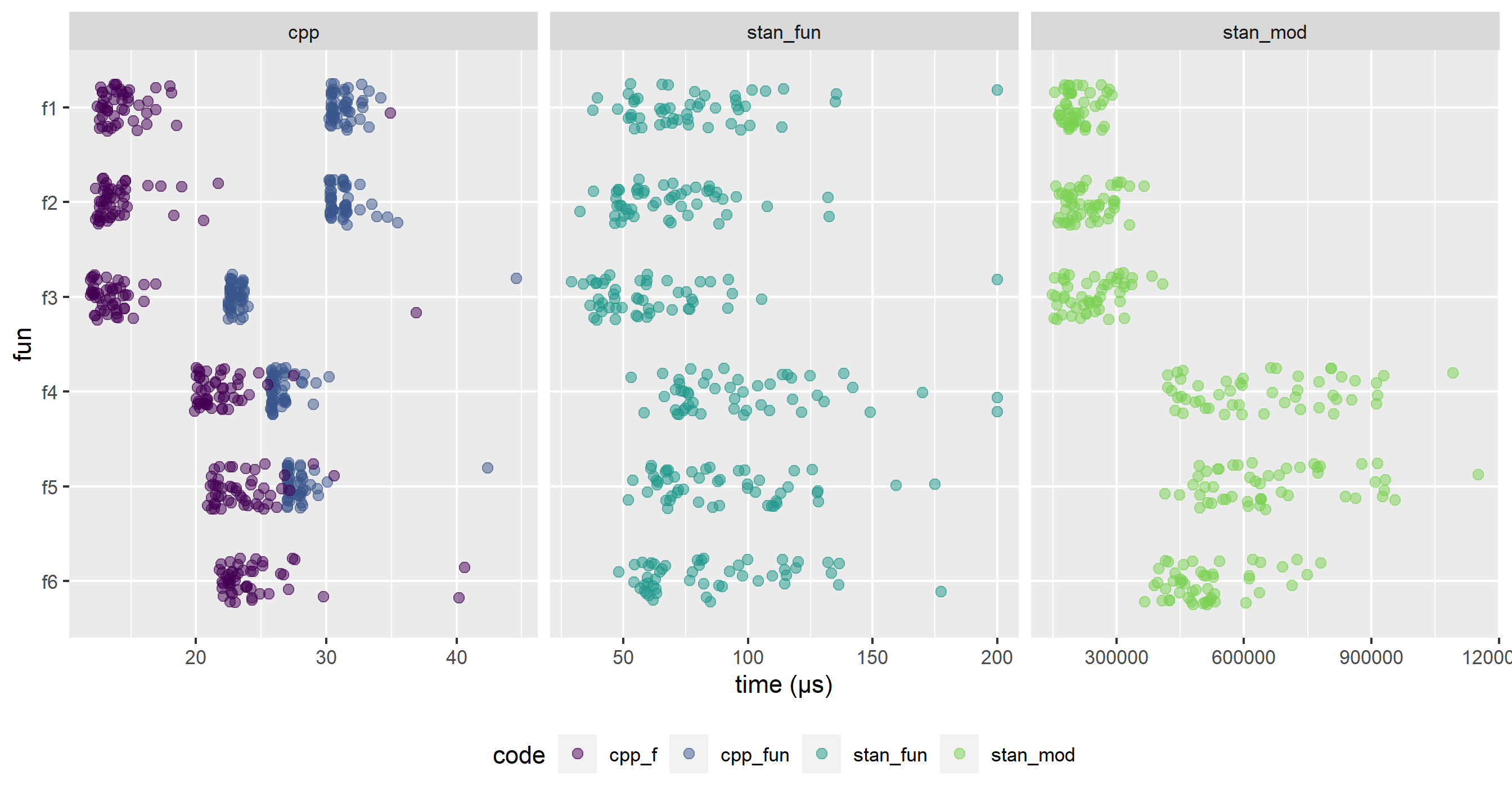
Resulting plot :

So with the original functions (cpp_fun), I thought the diminution in speed for fun[3:5] in Stan(stan_mod) as opposed to cpp was due to the way the functions log, exp and log1p were written. Instead of using directly std::log, std::exp and std::log1p, they add if…else & calls checks and on a loop that can add some time.

However, with the new function, even in cpp the f[4:6] do take longer both in cpp and stan.
I think the faster time for f[1:3] comes from defining double a = exp(log_alpha); m = exp(m); u = exp(u); so they don’t have to be recomputed every iteration.
Note : Another reason f3 is faster than fun3 in cpp and my f3 is faster in stan than ammd’s is because I removed 2 calls : f was log then exp when it could just be left as (exp(u) - exp(m)) / exp(m). (instead of log((exp(u) - exp(m)) / exp(m)) and then exp(f) on the next line.)

Related, re the last part of the last ammd reply :
f5 gets translated to m + log1p(exp(u + log(inv_logit(exp(log_alpha) x)))), so it has one more call than f3 and you log inv_logit(exp(log_alpha) * x) to then exp() it and then log() it again.

In cpp f5 is also half as slow than f3.

The cpp codes do run much faster. I know there are steps that aren’t done relating parameters, but I think part of this could be because of the vectorisation of functions. If I translate the cpp code to Rcpp which allows vectorisation instead of for loops, I do get much lower speed :/

2 Likes