Effect of declaring truncated distributions for parameters which already have a range declared

Hi, I have some parameters which look like

real <lower = L, upper = U> foo;

and then later in the model section,

foo ~ normal (mu, sigma);

I’ve been working with that for a while and it seems to have the expected effect, namely that the distribution of foo is truncated to the range [L, U]. Is it possible it’s not working correctly and I’m just fooling myself?

However, I’ve lately become aware that there’s a syntax for declaring a truncated distribution, such as

foo ~ normal (mu, sigma) T[L, U];

Given that there is already a range specified for the parameter, what is the effect of including T[L, U] in the distribution? Does it change the sampling distribution? Or perhaps it makes sampling more or less efficient? Or something else entirely?

Thanks for any insights. I’ve found some discussions about this topic in the Stan forums, such as Constraint checking and resulting distribution (truncated normal) - #2 by jsocolar , and also Sec. 7.4 in the reference manual (7.4 Sampling statements | Stan Reference Manual), but I’m not sufficiently enlightened to understand the implications for the case I’ve described here. I appreciate your help.

Robert Dodier
1 Like

What happens here depends on whether your bounds L and U are constants (data) or whether they are parameters (or they depend on parameters). If they are constants, then you’re fine (unless you are using Bayes factors to compare models with different constraints). If they are parameters, then you need the T statement.

Consider the following Stan program

parameters {
  real<lower=0, upper = 1> alpha;
  real<lower=0, upper = alpha> x;
}
model {
  x ~ uniform(0, 1);
}

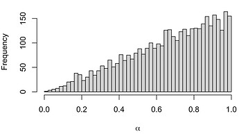
What we intend to have written is a prior on x that corresponds to the procedure: sample \alpha from a uniform distribution on [0,1], then sample x from a uniform distribution on [0,\alpha]. Thus we intend for this program to return a uniform margin for \alpha. But that’s not what happens:


What’s happening here is that conditional on \alpha being small, there’s only a small amount of posterior mass distributed over all allowable values of x. In other words, the posterior probability mass conditional on \alpha = 1 is properly normalized (i.e. integrates to 1), but conditional on other values of \alpha we aren’t normalized. Stan can drop normalizing constants, which is why this doesn’t matter as long as the bounds are constant. But here, the factor required to normalize the prior on x isn’t constant; it depends on \alpha. Thus it cannot be dropped. T[0, alpha] will tell Stan to normalize the prior.

5 Likes

Thanks a lot, that makes sense. In this case, L and U are indeed constants, so, as you were saying, T[L, U] doesn’t change the sampling distribution. However, I will keep it in mind for more general cases.

For some additional examples see also Section 6.2.2 of An Introduction to Stan.