I’m am trying to model the observed number of unique fossil species observed in geological units. The data are species counts for a specific unit during a specific time interval. There are 3 to 40 geological units observed in each time interval and 10 intervals. Each of the geologic units has 4 covariates of which the continuous variables are rescaled to have sd 0.5 and mean 0, the binary variables left as is, and one compositional variable resulting from a isometric log ratio transformed.
My goal with analyzing this data is to understand how average number of species per geological unit has changed over time, which time bins are particularly strange, and what if any relationship there is between the geological covariates and observed species diversity.
Because I’m modeling units which bear 1 or more fossil species, I’ve based on my model around a zero-truncated negative binomial distribution parameterized in terms of mean and dispersion (neg_binomial_2). The mean is modeled as a regression with both varying-intercept and varying-slopes while dispersion is assumed uniform through time. The group-level means for the varying-intercept and slopes are themselves given a random-walk prior. My justification here is that I’m looking at a sequence of time-bins and neighboring bins may be more similar than others. I’m using a non-centered parameterization for the model of the varying-intercept and slopes, as well as a non-centered parameterization of the random-walk prior.
data {
  int<lower=0> N;  // # observations
  int T;  // observation windows
  int K;  // number covariates

  int<lower=0> y[N];  // value observed
  int t[N];  // window for observation
  matrix[N, K] X;
}
parameters {
  matrix[T, K] mu_raw;  // group-prior
  //vector<lower=0>[K] sigma_mu;  // rw sd
  vector<lower=0>[K] sigma_mu;  // rw sd

  cholesky_factor_corr[K] L_Omega;  // chol corr
  matrix[K, T] z;  // for non-centered mv-normal
  vector<lower=0>[K] tau;  // scales of cov

  real<lower=0> phi;  // over disperssion
}
transformed parameters {
  matrix[T, K] mu;  // group-prior
  matrix[T, K] beta;  // regression coefficients time X covariate
  vector[N] location;  // put on right support

  // rw prior for all covariates incl intercept
  // this is non-centered which adds parameter but can improve sampling
  for(k in 1:K) {
    //mu[1, k] = 0 + sigma_mu[k] * mu_raw[1, k];
    mu[1, k] = mu_raw[1, k];
    for(j in 2:T) {
      mu[j, k] = mu[j - 1, k] + sigma_mu[k] * mu_raw[1, k];
    }
  }

  // non-centered mvn
  beta = mu + (diag_pre_multiply(tau, L_Omega) * z)';

  // matrix algebra
  location = exp(rows_dot_product(beta[t], X));
}
model {
  // rw prior
  to_vector(mu_raw) ~ normal(0, 1);
  sigma_mu ~ normal(0, 1);

  // effects
  to_vector(z) ~ normal(0, 1);
  L_Omega ~ lkj_corr_cholesky(2);
  tau ~ normal(0, 1);

  phi ~ normal(0, 0.5);

  for(n in 1:N)
    y[n] ~ neg_binomial_2(location[n], phi) T[1, ];
}
The model compiles fine, initializes fine, and fits one of my datasets (Brachiopoda) without worry with adapt_delta 0.99, stepsize 0.001, treedepth 15. However, when I try to fit the model to a different dataset (Bivalvia) I get a lot of divergent transitions. I get fewer divergent transitions when I push adapt_delta to 0.999 and stepsize to 0.0001, but still ~1% of my samples are divergent.
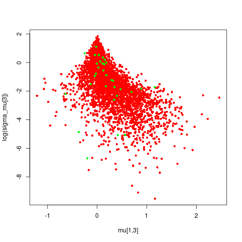
When I inspect the posterior samples from a few of my parameters the divergent samples don’t appear to have any particular pathologies; there is an obvious funnel but the divergent transitions appear fairly “random” wrt the tip of the funnel. I’m guessing these are false-positives but I’m not sure; perhaps the tip of the funnel has/needs more room to “grow”?

I have few questions that hopefully I can get help with:
1 - Should I just increase adapt_delta to 0.9999 and/or decrease the stepsize to 0.00001 to get rid of these divergent transitions? Or am I already pushing to limits of those options?
2 - Is there more I can do to improve my model that might help with this divergent transition issue?
3 - Have I implemented my random-walk prior correctly? I’m worried I’m missing something and have messed up the non-centered reparameterization.
Thanks very much. This forum and the mailing list before have been true life savers throughout my PhD and now into my current postdoctoral work.
stan file
trunc_test.stan (1.4 KB)
rdump
diversity_data_Brachiopoda.data.R (11.8 KB)
diversity_data_Bivalvia.data.R (7.0 KB)
bash script I use to run this model on two separate datasets using CmdStan:
#!/bin/bash
FILES=diversity_data_Brachiopoda.data.R
for f in $FILES;
do
  for i in `seq 1 4`;
  do
    trunc_test sample \
      adapt delta=0.999 \
      num_samples=5000 num_warmup=5000 thin=5\
      algorithm=hmc engine=nuts max_depth=15 stepsize=0.0001 \
      id=$i \
      init=0 \
      data file=$f \
      output file=trunc_${i}_Brachiopoda.csv &
  done
  wait
done
FILES=diversity_data_Bivalvia.data.R
for f in $FILES;
do
  for i in `seq 1 4`;
  do
    trunc_test sample \
      adapt delta=0.999 \
      num_samples=5000 num_warmup=5000 thin=5 \
      algorithm=hmc engine=nuts max_depth=15 stepsize=0.0001 \
      id=$i \
      init=0 \
      data file=$f \
      output file=trunc_${i}_Bivalvia.csv &
  done
  wait
done