I am modelling a dataset from a neuroscience experiment. When I’m trying to incorporate hierarchy in the model, I’m getting a few divergent transitions after warmup, for a variety of distribution families and model definitions. I would appreciate your advice on this; bellow I provide more information about my data and what I tried.
Experimental mice (N=4; total of ~11K trials) from a specific genetic strain were allowed to interact with mice from different genetic strains (CueID: a factor variable with six levels), and the dependent measure is the time they spent interacting (DwellTime: a strictly positive and heavily skewed variable). This first figure demonstrates that each mouse has a noticeable number of extreme observations:

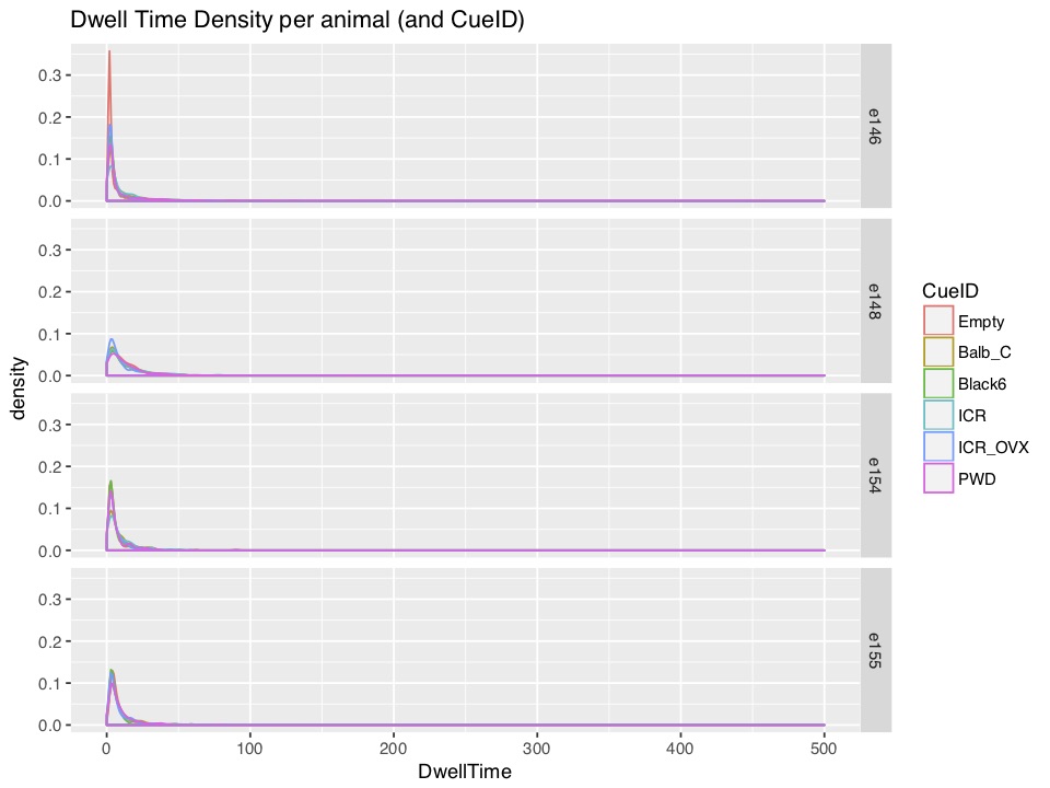
This second figure summarizes how
DwellTime looks in different conditions for each of the four mice.
My first step was to fit a regression model that predicts DwellTime using the CueID factor variable without any animal-specific terms:
post_DT_lognormal <- brm(formula = DwellTime ~ CueID,
                     data = big_dframe, family = lognormal(), warmup = 2000,
                     iter = 3000, chains = 4, control = list(adapt_delta = 0.98))
The diagnostics were fine and it seemed like the lognormal distribution did a good job; I tried also weibull(), Gamma(), gen_extreme_value(), frechet(), and exgaussian() families, but lognormal() mixed significantly fastest and had better loo log-likelihood.
When I introduced the next level of complexity, i.e., animal-specific intercepts:
post_DT_lognormal_mixeff_int_only <- brm(formula = DwellTime ~ CueID + (1 | AnimalID),
                                         data = big_dframe, family = lognormal(), warmup = 2000,
                                         iter = 3000, chains = 4, control = list(adapt_delta = 0.99, max_treedepth = 15))
I encountered a few divergent transitions after warmup (<10 across different attempts). Note that the model with the animal-specific intercepts had a better loo log-likelihood as compared to a population-effects only model.
                                                         LOOIC     SE
post_DT_lognormal_mixeff_int_only                     69595.29 312.75
post_DT_lognormal                                     70063.17 304.59
post_DT_lognormal_mixeff_int_only - post_DT_lognormal  -467.88  45.17
When looking at pairs(post_DT_lognormal_mixeff_int_only) () we see that the sd_AnimalID_Intercept term introduces a complex geometry with the other parameters (second column from right). If I understand correctly, brms implements a non-centered parametrization so this is probably not the problem.

And this isn’t solved when I try the other families that I mentioned above; It persists even when the model is in the simplified hierarchical form: formula = DwellTime ~ 1 + (1 | AnimalID), and moreover, when I trimmed outlier observations as well (and we wouldn’t like to throw these observations in any case).
Note also that when I log the data, it doesn’t look like a classic normal distribution, so not sure whether the log-normal distribution is the best here.

Similarly and as expected, when I introduce even more complexity and add animal-specific
CueID coefficients:
post_DT_lognormal_mixeff <- brm(formula = DwellTime ~ CueID + (CueID || AnimalID),
                                         data = big_dframe, family = lognormal(), warmup = 2000,
                                         iter = 3000, chains = 4, control = list(adapt_delta = 0.99, max_treedepth = 15))
I get 3 divergent transitions after warmup and similar geometric issues. Again, the model does a better job than the varying-intercepts model and ideally I would prefer it.
                                                                LOOIC     SE
post_DT_lognormal_mixeff                                     69460.41 313.12
post_DT_lognormal_mixeff_int_only                            69595.29 312.75
post_DT_lognormal_mixeff - post_DT_lognormal_mixeff_int_only  -134.88  22.25
Do you have any suggestions?
- Operating System: macOS Mojave 10.14.2,
- brms Version: 2.01
