Ok, here we go:
I hope this is not just some old Idea that has already been rejected due to some reason. However, it seems quite logical and natural to me and seems to work quite well, so I wondered why I didn’t see any mention of it, suggesting that it might actually hasn’t been considered before.
After I had this Idea I went looking for similar things in the forums an it turned out that @bertschi already proposed a very similar / the same solution here a few months back, also including some theory and a case study:
I can’t see much discussion of it, hovewer, or evidence that the idea has been picked up by the devs. Therefore I decided to highlight it again, which is the purpose of this thread. In addition, in that old thread some possibly interesting aspects remained undiscussed, and I’m also coming from a slightly different perspective.
I split this into two post. In this first post I present the basic idea, in the second post I discuss implementation.
First a simple example that highlights the problem.
Let’s say I have measured a bunch of angles and want to estimate the mean angle. I assume that the angles follow a von mises distribution. I parametrise the mean angle using an angle derived from a 2-dimensional unit vector via atan2().
Here’s the stan code of that model:
data{
    int n;
    real <lower=-pi(), upper=pi()> measuredAngles[n];
    }
parameters{
    unit_vector[2] meanAngleUnitVector;
    real<lower=0> precision;
}
transformed parameters{
    real<lower = -pi(), upper = pi()> meanAngle = atan2(meanAngleUnitVector[2], meanAngleUnitVector[1]);
}
model{
    precision~exponential(1);
    measuredAngles~von_mises(meanAngle,precision);
}
All model Runs in the following are conducted in the following way unless any deviations are mentioned:
They are fit via rstan 2.18.2 using the default settings (4 chains with each 2000 iterations, half of which is warmup). They are conducted on a simulated dataset of 100 measured angles coming from a von mises distribution with mean=1 and precision =3.
Running the model took 41 seconds (not including compilation) with a mean treedepth of 3.518 and produced 28 divergent transitions. (the previous run had >100 divergences).
Here’s the pairs plot:

As you can see there is some problem even with such a simple model.
The rest of this post is based on the assumption that I understood the implementation of the unit vector in Stan correctly. Based on what is written in the manual, and on forum posts. I understood it to work as follows:
If I declare a unit vector of dimension k, then Stan internally creates an unconstrained vector of dimension k and puts an independend standard-normal prior on each dimension. Samples of the unit vector are derived from this unconstrained vector by scaling each of them individually to length 1.
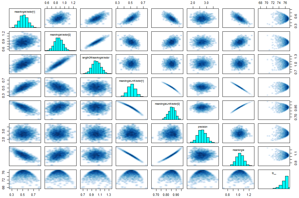
To be able to look at what happens inside this implementation I re-implemented the unit vector myself in the same way in my stan program. The program then looks like this:
data{
    int n;
    real <lower=-pi(), upper=pi()> measuredAngles[n];
    }
parameters{
    vector[2] meanAngleVector;
    real<lower=0> precision;
}
transformed parameters{
    real lengthOfMeanAngleVector = sqrt(meanAngleVector[1]^2+meanAngleVector[2]^2);
    vector[2] meanAngleUnitVector = meanAngleVector/lengthOfMeanAngleVector;
    real<lower = -pi(), upper = pi()> meanAngle = atan2(meanAngleUnitVector[2], meanAngleUnitVector[1]);
}
model{
    precision~exponential(1);
    meanAngleVector[1]~normal(0,1);
    meanAngleVector[2]~normal(0,1);
    measuredAngles~von_mises(meanAngle,precision);
}
Reassuringly, if I run this second model it produces an identical (within stochastic variation) runtime, treedepth and number of divergences as the first model (which used the native implementation of the unit vector).
Here’s the pairplot of the second model:

With this background, I now present my interpretation of what is going wrong there:
I think the key to understanding this, is to think about how the posterior distribution of the internal reprentation of the unit vector looks like. Its shape will on one hand be influenced by the internal standard-normal priors on each of its dimensions, and on the other hand by the other influences which are transmitted to it through the unit vector. As the unit vector contains no info about the length of the internal representations unconstrained vector, it can only transmit back information about the direction of the internal vector, not about its length.
In the following plot I simulate how this internal posterior density looks like when the information relayed back to it through its unit vector representation corresponds to a von mises density with precision=10. I calculated this density by multiplying the 2d-standard-normal prior density with the von mises density.

The point is exactly at the origin of the internal unconstrained vector.
It can be seen that the distribution is quite smooth away from the origin, but as one comes close to the origin it becomes sharper and sharper, leading to areas of fairly high curvature close to the origin (and a discontinuity exactly at the origin). I think these high curvature regions are what causes the divergences and/or treedepth issues.
So what causes the divergences seems to be the fact that due to the radial nature of the info relayed through the unit-vector, the originally smooth von mises distribution gets progressively "sharpened" towards the center of the internal unconstrained representation.
Here are two more examples.
The first uses a very narrow von mises distribution, simulating the posterior of a highly informative dataset. It agains shows how the curvature gradually increases towards the center. It can be seen that the posterior has a very sharp spike with high curvature edges, somewhat reminiscent of what is known as "neals funnel".

The second example uses a very broad von mises distribution, showing that a small problematic area always remains near the origin.

This illustrates that the issue should be worse if the angular distribution is sharper to begin with. Accordingly, the narrower the von mises distribution is, the slower the sampler, the higher the treedepth and the higher the change of divergences. Tho following plot illustrates this with model 2 (result for model 1 looked similar).

Plot explanation:
The von mises precision here describes the distribution of the measured angles in the simulated dataset. Each bar shows the distribution from 40 runs of 1 chain each, each run using a new simulated dataset. The width of each bar follows the empirical cumulative distribution function of the datapoints.
The solution Idea:
For the purposes of the unit-vector we use only the directional info of the internal unconstrained vector, not its length. This means that we are to some degree free to choose its length as we see fits. As can be seen from the plots above, problems with high curvature arise when the sampler is close to the origin, that is when the vector is short. Unfortunately, the current implementation uses standard-normal priors, which draw the sampler to this problematic region.
To avoid problems with the high curvature areas I suggest to change the prior of the unit vectors internal representation to one that keeps the sampler away from the these areas. I suggest that the typical set should not span much more than a 2-times difference in distance from the origin, such that the radial compression of the angular distribution can’t change the curvature by more than a factor of 2. This would present the sampler a relatively uniform amount of curvature, to which it can adapt well.
A simple prior that achieves this goal is if we replace the independend standard-normal distributions with one single normal(1,0.1) distribution that acts only on the length of the unconstrained vector (optimal choice and jacobian correction are discussed in the second post). This achieves a "donut" shaped distribution.
The following plots show the simulated shape of the posterior of the internal unconstrained vector. The plots are identical to the previous three ones, except that the prior has been changed from unit-normal to the "donut prior" suggested above.

Not the easiest distribution to sample from, but should be completely fine for Stan as it’s using HMC.

Here we can see that for highly informative datasets the posterior is very close to the shape of a multivariate normal. This should be very easy to sample from. If the density is even more narrow the distribution becomes a narrow ridge, but again, similar shape as a multivariate normal, so shouldn’t be a problem.

For a very uninformative dataset the distribution looks like a smoth ring. Again, not the most convenient distribution, but shouldn’t be a problem for HMC.
Implementing this into Stan model number 2 leads us to the following model number 3: (the only thing that has changed is the prior in the model block)
data{
    int n;
    real <lower=-pi(), upper=pi()> measuredAngles[n];
    }
parameters{
    vector[2] meanAngleVector;
    real<lower=0> precision;
}
transformed parameters{
    real lengthOfMeanAngleVector = sqrt(meanAngleVector[1]^2+meanAngleVector[2]^2);
    vector[2] meanAngleUnitVector = meanAngleVector/lengthOfMeanAngleVector;
    real<lower = -pi(), upper = pi()> meanAngle = atan2(meanAngleUnitVector[2], meanAngleUnitVector[1]);
}
model{
    precision~exponential(1);
    lengthOfMeanAngleVector~normal(1,.1);
    measuredAngles~von_mises(meanAngle,precision);
}
On a dataset like used for the first 2 models this run in 15 seconds, with mean treedepth of 2.3 and no divergences.
Here’s the pairplot:
Testing again for different concentrations of the von mises distribution:

The plot doesn’t show the strong relationship between runtime and distribution which appeared in the previous model, and there were no divergences. Update: I also tried it with much higher von-mises-precisions, and the runtimes stabilize at about 4.5 seconds.
Bob Carpenter once wrote that that the unit-vector was originally implemented to create a data structure where the points which are close together on e.g. a circle are also close together in its unconstrained representation. While the implementation achieves this goal, it unfortunately also puts close together such points which are not close on the circle. This is because all points of the circle are close together at the origin of the unconstrained representation. What the "donut-prior" achieves is that not only points that are close on a circle are close in the unconstrained representation, but also that points which should be far away from each other are so in the unconstrained representation, too. At least if we only consider the typical set, or the length of the path which the sampler typically travels between the points.
It also makes sense intuitively: If you want to model a circular variable, use a posterior that looks like a circle (donut). If you want to model coordinates on a sphere use a distribution shaped like (the surface of) a sphere, and so forth …