I’ve seen that there were several discussions about divergence/treedepth problems when using unit_vector for circular statistics in the past year.
E.g.:
Has this issue been resolved in the meantime?
If not, I think I might be able to explain the cause and give a solution. If there’s interest I can write It up and post some theory and a small case study here.
Go ahead. I think we know the cause, namely Euclidean-based HMC schemes can face weird geometry when trying to draw from posterior distributions that are defined on manifolds. And in particular with unit_vectors we originally were using a one-to-one but periodic transformation using polar coordinates and trigonometry but ran into the problem that 0 was far from 2 \pi in the unconstrained space. Then we switched to normalizing independent standard normals, which is better but isn’t quite one-to-one because the radius of the hypersphere is not really defined although we can take it to be 1 when converting initial values to the unconstrained space. It works well as a prior, but conditional on the data, it can have a weird shape. I’ve long thought that we could utilize the ambiguity about the radius to tune the sampler but if you have other solutions, feel free to post them.
I hope this is not just some old Idea that has already been rejected due to some reason. However, it seems quite logical and natural to me and seems to work quite well, so I wondered why I didn’t see any mention of it, suggesting that it might actually hasn’t been considered before.
After I had this Idea I went looking for similar things in the forums an it turned out that @bertschi already proposed a very similar / the same solution here a few months back, also including some theory and a case study:
I can’t see much discussion of it, hovewer, or evidence that the idea has been picked up by the devs. Therefore I decided to highlight it again, which is the purpose of this thread. In addition, in that old thread some possibly interesting aspects remained undiscussed, and I’m also coming from a slightly different perspective.
I split this into two post. In this first post I present the basic idea, in the second post I discuss implementation.
First a simple example that highlights the problem.
Let’s say I have measured a bunch of angles and want to estimate the mean angle. I assume that the angles follow a von mises distribution. I parametrise the mean angle using an angle derived from a 2-dimensional unit vector via atan2().
All model Runs in the following are conducted in the following way unless any deviations are mentioned:
They are fit via rstan 2.18.2 using the default settings (4 chains with each 2000 iterations, half of which is warmup). They are conducted on a simulated dataset of 100 measured angles coming from a von mises distribution with mean=1 and precision =3.
Running the model took 41 seconds (not including compilation) with a mean treedepth of 3.518 and produced 28 divergent transitions. (the previous run had >100 divergences).
As you can see there is some problem even with such a simple model.
The rest of this post is based on the assumption that I understood the implementation of the unit vector in Stan correctly. Based on what is written in the manual, and on forum posts. I understood it to work as follows:
If I declare a unit vector of dimension k, then Stan internally creates an unconstrained vector of dimension k and puts an independend standard-normal prior on each dimension. Samples of the unit vector are derived from this unconstrained vector by scaling each of them individually to length 1.
To be able to look at what happens inside this implementation I re-implemented the unit vector myself in the same way in my stan program. The program then looks like this:
Reassuringly, if I run this second model it produces an identical (within stochastic variation) runtime, treedepth and number of divergences as the first model (which used the native implementation of the unit vector).
With this background, I now present my interpretation of what is going wrong there:
I think the key to understanding this, is to think about how the posterior distribution of the internal reprentation of the unit vector looks like. Its shape will on one hand be influenced by the internal standard-normal priors on each of its dimensions, and on the other hand by the other influences which are transmitted to it through the unit vector. As the unit vector contains no info about the length of the internal representations unconstrained vector, it can only transmit back information about the direction of the internal vector, not about its length.
In the following plot I simulate how this internal posterior density looks like when the information relayed back to it through its unit vector representation corresponds to a von mises density with precision=10. I calculated this density by multiplying the 2d-standard-normal prior density with the von mises density.
The point is exactly at the origin of the internal unconstrained vector.
It can be seen that the distribution is quite smooth away from the origin, but as one comes close to the origin it becomes sharper and sharper, leading to areas of fairly high curvature close to the origin (and a discontinuity exactly at the origin). I think these high curvature regions are what causes the divergences and/or treedepth issues.
So what causes the divergences seems to be the fact that due to the radial nature of the info relayed through the unit-vector, the originally smooth von mises distribution gets progressively "sharpened" towards the center of the internal unconstrained representation.
Here are two more examples.
The first uses a very narrow von mises distribution, simulating the posterior of a highly informative dataset. It agains shows how the curvature gradually increases towards the center. It can be seen that the posterior has a very sharp spike with high curvature edges, somewhat reminiscent of what is known as "neals funnel".
This illustrates that the issue should be worse if the angular distribution is sharper to begin with. Accordingly, the narrower the von mises distribution is, the slower the sampler, the higher the treedepth and the higher the change of divergences. Tho following plot illustrates this with model 2 (result for model 1 looked similar).
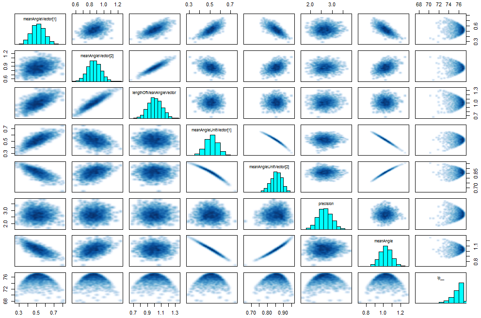
Plot explanation:
The von mises precision here describes the distribution of the measured angles in the simulated dataset. Each bar shows the distribution from 40 runs of 1 chain each, each run using a new simulated dataset. The width of each bar follows the empirical cumulative distribution function of the datapoints.
The solution Idea:
For the purposes of the unit-vector we use only the directional info of the internal unconstrained vector, not its length. This means that we are to some degree free to choose its length as we see fits. As can be seen from the plots above, problems with high curvature arise when the sampler is close to the origin, that is when the vector is short. Unfortunately, the current implementation uses standard-normal priors, which draw the sampler to this problematic region.
To avoid problems with the high curvature areas I suggest to change the prior of the unit vectors internal representation to one that keeps the sampler away from the these areas. I suggest that the typical set should not span much more than a 2-times difference in distance from the origin, such that the radial compression of the angular distribution can’t change the curvature by more than a factor of 2. This would present the sampler a relatively uniform amount of curvature, to which it can adapt well.
A simple prior that achieves this goal is if we replace the independend standard-normal distributions with one single normal(1,0.1) distribution that acts only on the length of the unconstrained vector (optimal choice and jacobian correction are discussed in the second post). This achieves a "donut" shaped distribution.
The following plots show the simulated shape of the posterior of the internal unconstrained vector. The plots are identical to the previous three ones, except that the prior has been changed from unit-normal to the "donut prior" suggested above.
Here we can see that for highly informative datasets the posterior is very close to the shape of a multivariate normal. This should be very easy to sample from. If the density is even more narrow the distribution becomes a narrow ridge, but again, similar shape as a multivariate normal, so shouldn’t be a problem.
For a very uninformative dataset the distribution looks like a smoth ring. Again, not the most convenient distribution, but shouldn’t be a problem for HMC.
Implementing this into Stan model number 2 leads us to the following model number 3: (the only thing that has changed is the prior in the model block)
The plot doesn’t show the strong relationship between runtime and distribution which appeared in the previous model, and there were no divergences. Update: I also tried it with much higher von-mises-precisions, and the runtimes stabilize at about 4.5 seconds.
Bob Carpenter once wrote that that the unit-vector was originally implemented to create a data structure where the points which are close together on e.g. a circle are also close together in its unconstrained representation. While the implementation achieves this goal, it unfortunately also puts close together such points which are not close on the circle. This is because all points of the circle are close together at the origin of the unconstrained representation. What the "donut-prior" achieves is that not only points that are close on a circle are close in the unconstrained representation, but also that points which should be far away from each other are so in the unconstrained representation, too. At least if we only consider the typical set, or the length of the path which the sampler typically travels between the points.
It also makes sense intuitively: If you want to model a circular variable, use a posterior that looks like a circle (donut). If you want to model coordinates on a sphere use a distribution shaped like (the surface of) a sphere, and so forth …
“I suggest that the typical set should not span much more than a 2-times difference in distance from the origin, such that the radial compression of the von mises distribution (or whatever other angular distribution) can’t change the curvature by more than a factor of 2. This would present the sampler a relatively uniform amount of curvature, to which it can adapt well.”
The proposed normal(1,0.1) prior on the vector length was chosen according to this rule. If we make the ring too broad this will not solve the problem in full, leading to higher than optimal treedepth and running time, and a risk of divergences. If we make it much narrower, the sampler would also have to make smaller steps to navigate the distribution, which wouldn’t lead to divergences, but make it slower. So besides the desire to avoid divergences, this is primarily a question of what gives optimal performance.
We might also discuss what the optimal shape of the donuts flanks may be, although I think the normal distribution is probably already the optimal choice. But on theoretical grounds it would be desireable to have a prior that completely forbids the sampler to go to the origin, which the normal distribution doesn’t do.
We should also think of what happens in higher dimensions. While in low dimensions the current implementation of the unit vector draws the sampler towards the origin, in higher dimensions this is offset by the proportionately much lower volume there, so that the sampler rarely goes there. Therefore I suspect that the current implementation already works well for high-dimensional unit-vectors, and only low dimensions show the problematic behaviour. Something I didn’t test because I’m not very firm with higher dimensional calculations.
Another question is how the proposed "donut-prior" may behave in high dimensions. I suspect that the ring would probably increase in radius and become narrower, which may or may not be optimal for performance.
When @bertschi suggested this same Idea a few months ago he proposed to apply a jacobian correction to the “donut prior” (he used exactly the same “donut prior” as I did). He only provided the jacobian for the 2-dimensional case, where it is 1/vectorLength. I think the general form is vectorLength^(1-dimension). This jacobian correction effectively prevents that the ring icreases in radius or narrows with increasing dimension, possibly ensuring optimal performance for all dimensionalities. There are also some potential problems with this jacobian, however. Maybe @bertschi can say something about his experiences with that, I didn’t test it. So, based on theory, the following points might speak against using the jacobian:
it increases the density near the places where the high curvature lies (around the origin), increasing the chance that the sampler goes there.
it creates new high curvature shapes by itself (only around the origin).
it creates a very small very high target-density (not posterior-density) region (around the origin), which means that the sampler could get stuck there. This might act like what is known as a “phase change”. I don’t have any experience with how HMC acts when it gets in such a situation, but guess that it would either lead to a lot of rejections/divergences, or bad exploration, depending on the adaptation.
it creates one point with infinite density (the origin).
In practice, the jacobian might in fact be totally unproblematic, as due to the combined effect of the dimensionality (which exactly cancels out with the jacobian) and the "donut-prior" the sampler will be unlikely go near the origin anyway, and even if it does, most the target-density spike near the origin is not very high compared to the target-density of the donut. The exception beeing if the chain is initialised there, but as far as I understood the unconstrained representation of unit vectors is by default initialised with length 1 (is that true?).
The following plot shows the target (not posterior) density of the combination of the "donut-prior" with the jacobian for the two-dimensional case in black, and the 4-dimensional case in red. Note that the y-axis has a log-scale.
One point that I’m not sure about is how the jacobian might behave numerically or interact with the sampler in high dimensions, as I think the strength of the jacobian grows very fast with dimension. (How many dimensions might a unit-vector maximally have in practice?)
It might be that all possible variants work just fine. In that case it’s just a matter of performance optimisation. In this case some of the things to keep in mind are to keep treedepth at minimum, and to minimize the time required to derive the gradients.
I hope these 2 posts raise some useful points and apologise for the abuse of the words "donut" and "prior".
This looks promising. The Stan language is in the process of getting these “multiplier” keywords (really just scalings) for non-centered parameterizations. Perhaps we could have something similar for unit_vectors like
thanks for the detailed and very interesting analysis.
Let me quickly comment on the Jacobian. When going from the unconstrained space to angular coordinates, the density is transformed by the Jacobian of the change of coordinates. Thus, in order to ensure that the vector length r has indeed a (truncated) Gaussian distribution, we need to correct for the change of measure. Here, we only care for the uniform distribution on the angles and could simply ignore the correction for the length. I don’t know what the induced density on the length would be in that case, but from some quick experiments it seems to avoid zero more strongly while being more heavy tailed than the Gaussian. This all appears to be consistent with your density plot … the singularity arises because the Gaussian is truncated and does not pull the density towards negative infinity. In any case, I would keep the Jacobian as the model density is fully known in this case, but use another distribution in order to constrain the length. E.g. a log-normal with mean 1 would prevent the singularity as its density drops faster towards zero than it is pulled up by the Jacobian.
Transforming to angular coordinates is more involved in higher-dimensions, so I consider only polar coordinates in my write-up. It appears correct that the Jacobian for the d-dimensional case is given by r^{d - 1} when only the vector length needs to be controlled, I have not thought it through completely. The standard Gaussian density on the unconstrained space should be unproblematic though from dimension d >= 3 onwards. In this case, the vector length has an induced chi distribution with d degrees of freedom. The chi density is essentially r^{d - 1} e^{-1/2 r^2}, i.e. a standard Gaussian transformed by the Jacobian above (meaning it should be correct). Only for d = 2 the chi density does not vanish at r = 0. It might still make sense to constrain the vector length somewhat more strongly. I have not played with different choices for densities on r, especially not with the idea of finding an optimal width for the donut that Stan has to sample from. Would certainly be interesting to explore a bit more in this direction, e.g. using log-normal, Gamma or other distributions supported on positive real numbers to keep the vector length r close to unity.
Yes, I could imagine that a good solution might be to keep the current multivariate normal approach for high dimensions, and use the “donut prior” only for low dimensional cases. But I’m not sure.
I don’t know why exactly, but it’s often being said that the normal distribution is easiest for the sampler. This this is probably a bit different if we bend the distribution to form a ring, but I suspect the optimal distribution for that use case would still be roughly similar to a normal distribution.
Here’s a plot of two different densities for various dimensions:
the densities used are:
normal_lpdf(distance|1,0.1) (the donut)
normal_lpdf(log(distance)|0,0.1)
Nice, I assume all densities include the Jacobian term and the solid lines are for the normal and the dashed for log-normal?
Don’t think that normal distributions are much easier for HMC than others. My reasoning was simply to prevent the sampler from reaching zero where problems arise and at the same time keep it from wandering around too far. Its probably best for HMC if all parameters have a similar scale and the curvature does not change much across the space. Thus, I considered the normal prior as a soft constrained on the vector length which keeps it somewhat close to unity. Don’t know if unity is any better here than other values, but heavy tails should be good as it keeps the sampler from moving far out. As the likelihood does not add any information on the vector length, we are free to choose any prior that allows for easy and efficient exploration of the donut in the unconstrained space.
Exactly!
I should also mention again that the plot shows the target density, not the density of the resulting samples (which would cancel out the yacobian term).
This would be a great paper for StanCon. We’d also be happy to publish it as a case study along with our doc, but maybe it makes more sense as just something to motivate changing our underlying representations. But in that case, I still think it would be a very useful computational stats paper in and of itself. I’d be happy to provide comments.
As you verified, you were right about how our unit vector is coded.
That’s the key to all sampling in Stan! It’s all in the posterior geometry.
Yes, that’s exactly what’ll happen in that posterior. Any time we get varying curvature between very flat surfaces and high curvature, we run into problem with not being able to find a good global adaptation for step size.
This is really hlepful for diagnosing the problem. We should’ve done this ourselves!
This is also what worked for us in a case of spatial models where we had a sum-to-zero constraint on random effects. If we put a hard constraint:
then we find the same sort of geometric problems. But when we change that constraint to a soft constraint, the posterior geometry is less sharp and the sampler works an order of magnitude faster.
The scale of the normal varies with the problem, and we don’t have a good idea of what to recommend to start.
The problem with donuts is that they also have varying curvature. But our adaptation should be able to deal with mild conditioning like this OK by just taking smaller step sizes.
Is there a way we could unwind that donut?
Yup. I didn’t realize that was so bad!
Nice—it concludes with a folk theorem for solving the folk theorem!
We tried that in 2012 and ran into the problem that 0 and 2\pi were far apart in the unconstrained space, which is why we changed the underlying parameterization of unit_vectors to what it is now. You can unwind it in a different way
but then \infty and -\infty in the unconstrained space both map to the same point in the constrained space, so that region has to have no posterior volume.
Just played a bit with different distributions and it appears that log-normal or Gamma would both be more reasonable than the truncated normal. All plotted distributions have unit mean and standard deviation of 0.1. Would probably take the Gamma(shape = 100, rate = 100) if I had to choose.
I’d be happy to contribute. From my perspective combining makes more sense than writing something alone, because this would provide context, making it more “complete”. It would be difficult for me to achieve that on my own.
I’m not sure if I can follow you there. I understand that If we look at the two dimensions of the donut independently they have varying curvature, but from the perspective of the full 2-dimensional structure it should be almost uniform (although anisotropic), right? (except in the center, of course). Having it uniform in 1d would be nicer of course, but if this is not possible making it uniform in 2d is probably the next-best solution.
Of course, if we change the truncated normal to a log-normal or gamma this might decrease uniformity, while the yacobian might as well in theory, but in practice might effectively improve it (by correcting for the curvedness of the donut, helping the sampler to get around the curve). I’d have to think more about that.
Well, not trying to unwind it is exactly what lead to this solution, so maybe we just have to deal with that. Because if we unwind it we probably get the problem with the topology mismatch again. The nice thing about the donut is that while it’s living in a space that doesn’t match he topology of the circular variable, the shape of the donut actually kind of does match it, thus kind of circumvents the topology mismatch problem.
That said, given single-variable representation of a circular parameter, I don’t quite understand why one can’t just project the leapfrog position over to the other side when the sampler leaves the boundary of the circular variable (e.g. -pi to pi). So e.g. when the leapfrog jumps to -pi-0.123 move it over to pi-0.123, keeping the momentum the same. Intuitively I’d think that this would work fine with HMC, but might be problematic for NUTS because it might break the detection of U-turns? I think such a solution would be ok for the R^ and n_eff computations, as these values look ok at first sight for the angle derived from the donut-representation.
Doesn’t that also produce the same problem as just using the space from 0 to 2pi, that the endpoints are not connected?
Yes, although infinity is a better place for that to occur than anything finite. Still if your constrained point could be near -1, then it won’t work well.
I’d be happy to contribute as well. Maybe we could start with a case study and then expand into a more complete computational stats paper. As a starting point, we could compare different ways to represent the unit sphere as discussed here.
From what I understand, it is not possible to faithfully represent an angle with a 1-dimensional Euclidean parameter due to its circular geometry. The same would be true for the unit sphere in higher dimensions. Instead, such objects can be embedded into an Euclidean space of higher dimension, i.e. as done here with a unit vector in a d+1 dimensional space. Then, one could either impose a hard constraint to stay exactly on the d-dimensional subspace corresponding to the unit sphere or a soft constraint to keep the sampler close to it. The mathematically proper way for handling the hard constraint in HMC seems to be discussed in this paper Geodesic Monte Carlo on Embedded Manifolds - PMC.
This would require to change the internals of the sampler, as the integration of the Hamiltonian has to be projected back onto the subspace in each step. The soft constraint, as discussed above, could be added without such changes. Here, the sampler is free to move in \mathbb{R}^{d+1} while the length of the vector is contained by a suitable prior, e.g. the Gamma suggested above. Don’t know which method works better in practice, but both should be an improvement over the current implementation where the soft constraint is too weak except in high dimensions.
Don’t think there is a silver bullet with respect to the curvature. In the end, the sampler has to run around the origin in order to traverse the angular space. At a larger radius the curvature will be reduced, yet the distance/scale that needs to be travelled increases. Maybe there is an optimum for the width of the donut though?
This is an excellent review of the situation. The changes required for implementing non-Euclidean parameter spaces are surprisingly comprehensive. Not only would the integrator have to change but also the storage of all of the parameters would have to change to separate them into their varying topologies. Even with all of that many of the diagnostics and default chain output would have to change because means, variances, and quantiles are no long uniquely defined on non-Euclidean spaces.
I’ve never heard the term “anisotropic”, so had to look it up. I just mean that if we have a donut, then the second derivative matrix varies around the posterior. Maybe it doesn’t—it won’t in the hyper-donut defining the typical set for the normal, for instance.
Thsi would all break our simple Euclidean NUTS in R^N. You could do that wrapping with custom samplers—it just won’t work with Stan as currently written. People have built HMC to work directly on hyperspheres [I see the Byrne and Girolami geodesics paper—Simon Byrn’s the one who did a lot of this work]. @betanalpha has written about how to translate NUTS to more general manifolds, so we can also have that. It just needs custom code for everything and it wouldn’t be clear how to integrate it with Stan’s sampler.
To help deciding on an implementation I did some more tests to find out what donut shape is optimal, and whether to use the jacobian.
Test 1:
I tested two cases: highly informative likelihood (->narrow posterior angular distribution) and completely uninformative likelihood (->complete donut). The first test is to check the occurrence of divergences due to the radial sharpening of the likelihood through the circular projection, the second test is to check how fast the sampler can navigate the donut. It turned out that even in the second test divergenges can occur, more on that below.
I tested both conditions with all three proposed donut shapes (normal, lognormal, gamma), with and without jacobian, and with various widths of the donut. The mean of the donut prior (the “donut-radius”) was always approximately 1.
For the test of the uninformative likelihood I just left the likelihood away completely.
For the test of the highly informative likelihood I fixed the von mises precision parameter to 300 and fed the model 15 datapoints from a von mises distribution of this precision. I turns out that this produces approximatively the same posterior shape as in my first bunch of tests (posted above) with 100 datapoints and von mises precision 300, because the precision prior in the first tests was quite stupid and led to a very biased precision estimate (~42), which made the likelihood wider than it would otherwise have been (which doesn’t matter beacuse I didn’t rely on it anywhere). As in the first tests the performance and divergence figures stabilized at precision 300 and didn’t change much for higher precisions, the test at this value should be ±representative for “infinite” precision likelihoods.
All tests were repeated 100 times with new random datasets.
Plot explanation:
The x-axis shows what donut-shape was used. The first number on each colum denotes which distribution was used (1=normal, 2=lognormal, 3=gamma) and the second number tells whether the jacobian was applied (0=no 1=yes). Everything else is as in the graphs in my posts further up.
Results summary:
Even if the likelihood is completely uninformative (in the test I just removed the likelihood altogether) there can be divergences. I think this can be due to two reasons:
for the zero-avoiding distributions if the sampler gets too close to zero there is a crazy gradient.
in any case if the sampler manages to ±completely leapfrog over the region around the origin the hamiltonian integration is probably very bad (not sure if this would lead to a divergence warning as I don’t know exactly how divergences are detected).
Within the range of values tested, for uninformative likelihoods broad donuts are faster (easier to navigate for the sampler), for informative ones narrow ones are faster (because it decreases the radial sharpening of the likelihood). Outside the tested range other effects can apply, but this range is not interesting for our purpose (at the moment).
But for the sake of completeness:
For uninformative likelihoods if the donut-sd is >0.3 it seems to stop getting faster and at some point actually gets slower again, didn’t test this much. Presumably this is because the sampler then gets more often to the problematic central part of the distribution (but if sd>>0.3 then this doesn’t register as divergences). We can already see that starting at 0.3 in the plot. The special case of the normal-donut without jacobian might be ±immune to this.
For higly informative likelihoods I suspect that if the donut-sd is made very small then the warmup time will increase again because it takes time to find the correct scale for the sampler (didn’t test).
The initially chosen donut width of sd=0.1 seems to be close to optimal.
With highly informative likelihood the lognormal is best, followed by the gamma and then the normal. Applying the jacobian makes the results worse. Without the likelihood it’s all reversed. Overall it doesn’t make much differnce which of the distributions is chosen, and whether the jacobian is applied. This might be different in higher dimensions (especially for the jacobian), here I tested only the two-dimensional case.
Discussion:
In real applications the energy distribution might vary (is this true?). Not sure what effect this would have, but I guess it might help the sampler to move into the problematic reagions, thus increasing the chance of divergences or increase of treedepth.
In real applications the shape of the angular distribution might be less “nice” than the Von Mises, also increasing the risk of divergences etc. . Such a less nice distribution could, amongst other things, also arise from the interaction with other model parameters, e.g. the estimate of the precision of the von mises might be uncertain, leading to a “neals funnel” type problem.
For these reasons it might be wise to err on the safe side and choose a narrower donut than sd=0.1*radius. Although, of course, this might be foregone in the sake of performance. If issues with divergences occur this can be countered by increasing the acceptance target.
I’m not quite sure if, in this special case, divergences do signal a bias in the posterior. I suspect that they do cause a bias because they alter the number of possible pathways between different parts of the posterior angular distribution, and thus the probability of moving from a certain angle to a certain other angle.
Test 2:
I also partly tested the effect of the jacobian in higher dimensions. I used the normal(1,0.1) donut-prior and left away the likelihood (because im not knowledgeable in higher dimensional angular math).
As expected, the length distribution of the vector grows with dimension without jacobian, and is stable with jacobian:
If we ignore the strange pattern It seems that performance in high dimensions is good and that, again, it doesn’t matter much whether the jacobian is applied or not, at least till 128 dimensions. With the yacobian I couldn’t go to 256 dimensions, because then initial values were rejected. I guess the jacobian just puts out too crazy numbers in that case. Without the jacobian it is possible to go higher.
(edit: What happened to the colours of the last 2 images?)