I’m just doing this for fun, so advice is welcome but not at all urgent.
A paper titled “2D Bayesian automated tilted-ring fitting of disk galaxies in large HI galaxy surveys: 2DBAT” showed up on arxiv.org a few weeks ago that addressed a problem I’ve been thinking about off and on for a while. I liked the idea of what the authors are doing, but I didn’t like the implementation. So I decided to try my own in Stan. If you take a look at the paper equations 1-4 describe the model; I’d suggest not reading past section 3.1.
For a little bit of context disk galaxies are usually assumed to be round, with stars and gas in more or less circular orbits around the center. If a galaxy is inclined to the plane of the sky it appears elliptical – assuming it’s actually round you can deduce the inclination angle. The other relevant angle is the orientation on the sky, which is conventionally defined to be the angle measuring counterclockwise from north to the apparent major axis. With spatially resolved spectroscopy you can measure a 2D field of radial velocities – the data I have came from SDSS-IV MaNGA. The problem is to derive the rotation curve from the velocity field.
Here is my current Stan model, which slightly simplifies the model described in the paper:
functions {
  real sump(vector c, real r, int order) {
    real s = c[1];
    for (i in 2:order) {
      s = s + c[i]*r^(i-1);
    }
    return s;
  }
}

data {
  int<lower=1> order;  //order for polynomial representation of velocities
  int<lower=1> N;
  real x[N];
  real y[N];
  real v[N];  //measured los velocity
  real dv[N]; //error estimate on v
  int<lower=1> N_r; //number of points to fill in
  real r_post[N_r];
}

parameters {
  unit_vector[2] phi;
  unit_vector[2] incl;  //disk inclination
  real x_c;  //kinematic centers
  real y_c;
  real v_sys;     //system velocity offset (should be small)
  real v_los[N];  //latent "real" los velocity
  vector[order] c_rot;
  vector[order] c_exp;
  real<lower=0.> sigma_los;
}

transformed parameters {
  real<lower=0.> r[N];

  for (i in 1:N) {
    r[i] = sqrt((-(x[i] - x_c) * phi[1] + (y[i] - y_c) * phi[2])^2 +
                (((x[i] - x_c) * phi[2] + (y[i] - y_c) * phi[1])/incl[2])^2);
  }
}

model {
  x_c ~ normal(0, 2);
  y_c ~ normal(0, 2);
  v_sys ~ normal(0, 50);
  sigma_los ~ normal(0, 20);
  for (i in 1:order) {
    c_rot[i] ~ normal(0, 100);
    c_exp[i] ~ normal(0, 100);
  }

  for (i in 1:N) {
    v[i] ~ normal(v_los[i], dv[i]);
    v_los[i] ~ normal(v_sys + incl[1] * (
                      sump(c_rot, r[i], order) * (-(x[i] - x_c) * phi[1] + (y[i] - y_c) * phi[2])  +
                      sump(c_exp, r[i], order) * (-(x[i] - x_c) * phi[2] - (y[i] - y_c) * phi[1]) / incl[2]),
                      sigma_los);
  }
}

generated quantities {
  real v_rot[N];
  real v_exp[N];
  real v_model[N];
  real vrot_post[N_r];

  for (i in 1:N) {
    v_rot[i] = fabs(r[i]*sump(c_rot, r[i], order));
    v_exp[i] = r[i]*sump(c_exp, r[i], order);
    v_model[i] = v_sys + incl[1] * (
                      sump(c_rot, r[i], order) * (-(x[i] - x_c) * phi[1] + (y[i] - y_c) * phi[2])  +
                      sump(c_exp, r[i], order) * (-(x[i] - x_c) * phi[2] - (y[i] - y_c) * phi[1]) / incl[2]);
  }
  for (i in 1:N_r) {
    vrot_post[i] = fabs(r_post[i] * sump(c_rot, r_post[i], order));
  }
}
I quickly discovered that making the two relevant angles parameters won’t work, so those are both declared as 2D unit vectors instead. The velocities are measured with error and I have estimates for the uncertainties, so I follow the measurement error discussion in the Stan language manual and model the observations as coming from normal distributions with unknown means and known standard deviations. Those latent means are then modeled as coming from a gaussian with mean described by equations 1-3 in the arxiv paper and for simplicity constant variance, which I model.
I decided to declare the deprojected radius in the transformed parameters block. I also tried declaring it as local variables in the model block but it seemed to make no difference to performance. The other parameters in the model are the cartesian coordinates of the kinematic center, which should be small adn the overall system radial velocity which should also be small (velocities are measured relative to the overall system redshift). The authors of the arxiv paper used splines for the radial and peculiar velocity components. For a first pass I just use a low order polynomial, so the coefficients are the parameters.
I’ve tried this on 3 data sets so far and it works, but it’s very fragile. I find I have to fiddle the target acceptance rate and maximum treedepth – setting adapt_delta in the range 0.95 - 0.975 and max_treedepth=15 usually works. It often takes several runs with different random initializations to get reasonable looking results, but it isn’t too difficult to tell when the results look reasonable.
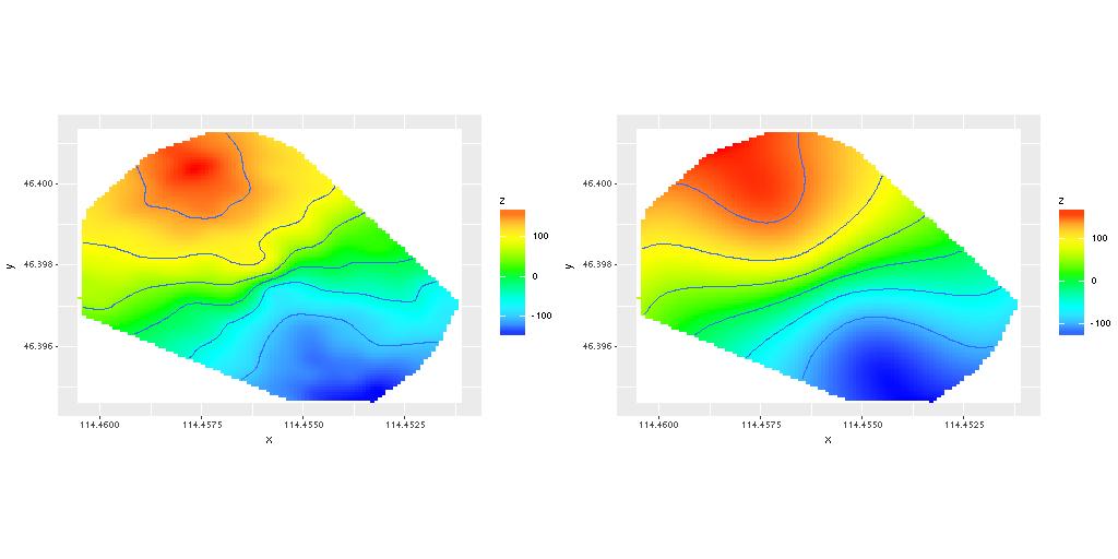
Here are some results from one successful run. First the measured velocity field and the (posterior mean) modeled velocities:
The thing you’re most interested in is the rotation curve. Here is the joint density of the deprojected radius and rotation velocity:

Both the magnitude and shape of the curve are very reasonable, but I haven’t seen independent estimates in the literature for this particular galaxy.
Here’s one traceplot for the first element of the parameter phi:

These are inherently multimodal and in this run fortunately both modes were discovered well within the warmup period.
Questions:
-
Is there an obvious reparametrization of this model that would make it less fragile?
-
The general “tilted ring” model allows the inclination and orientation angles to vary with radius, and the arxiv paper uses splines for that purpose. I don’t see an obvious way to do something equivalent with unit vectors.