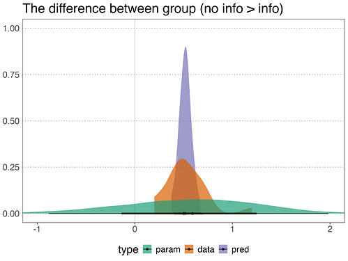
Differences in uncertainty (interval width) between model parameters and posterior predictions

I’m using a cumulative probit model with Likert data. For this post, I’ve simplified things, in terms of the model structure and the amount of data (I only used ~10% of the data). The model includes varying item thresholds, as well as varying intercepts for items and participants. Model formula as follows:

formula = bf(use | thres(4, gr = item) ~
1 + group +
(1 | item) +
(1 | pid))

Abbreviations: use = dv on a 1-5 likert sale; item = image to be rated; group = between participant categorical factor; pid = participant id.

I tried to attach the reprex model object (model bf.rds), but the forum didn’t allow the file type. Anyway, maybe my question can be answered without it and based on some principles.

My main question is as follows. It might be fairly basic, as I am inexperienced with these types of model (and most other models, for that matter). In short, the interval estimate for the fixed effects parameter estimate for my main predictor (group: a between participant categorical predictor that indexes the key experimental manipulation) is considerably wider than the interval estimate of the posterior predictions for the same between group difference (see figure below; param = fixed effect of group from the parameter in the model; data = data; pred = posterior predcition via tidybayes add_epred_draws()).

In the past, when I’ve been using other, simpler models, I have not seen such discrepancies between fixed effects and posterior predictions. From what I’ve read (with the possible caveat that I have a bug in my code), my current (mis)understanding goes something like this: the posterior predictions are formed by combining the sum total of parameters in the model, rather than just the fixed effects. And in this model, there are a whole bunch of parameters. For example, in this toy dataset, there are 20 items, each of which has 4 thresholds. And there are 10 pids per group. However, I think I’m still missing an intuition and a justification for why the interval estimates are so discrepant. And this matters, in terms of communicating uncertainty and drawing conclusions, because in one case, the inference would be uncertain as to the sign of the effect (as the interval would cover negative and positive values). In the other case, it would be reasonably certain about the sign (entirely positive). To put it in the crude terms that Reviewer 2 would surely use: “In one case, you show a clear effect of group, whereas on the other case, you do not. What’s going on?”

I would appreciate any help clarifying this matter. And I fully expect I could be confused on multiple levels.

And a more general question about the forum: is there a way to upload a model object to this forum?

FInally, if the data and code help, then I can supply them. But maybe let’s see if the question can be answered first without them.

Thanks.

  • Operating System: Mac OS sonoma 14.5
  • brms Version: brms 2.21.0

Can you show the code you used to generate the predictions, the parameter posterior draws, and the plot?

Note also that add_epred_draws gives you the posterior expectation (the predicted average value, excluding residual variance) and will therefore have a narrower distribution than the posterior predictions for a specific observation (which you would extract with add_predicted_draws).

Sure thing. It might be easier (by using less code) if I just show you how I would make quantile intervals, then I can save showing you how I made the plots. e.g., the quantile intervals will give you the same sense of the difference in interval width.

And yes, I know what you mean about the differences between add_epred_draws() and add_predicted_draws(). After your comment, I also used as_predicted_draws() below for comparison. As you can see, they are borader than epred draws (as you would expect), but they are still very similar to epred draws. And both types of predictions are very different from the interval width of the parameter posterior draws. I hope that’s not overly confusing.

Anyway, I hope the code below makes sense. It uses tidyverse wrangling and tidybayes functions. It may well be inefficient and/or confused. Sorry about that. But thanks so much for helping. The model is named “bf”.

## for the model parameter estimates for the effect of "group"
## fixed effect of group (minus per item thresholds)
post_qi_fix <- as_draws_df(bf) %>%  #
  as_tibble() %>% 
  select(starts_with("b_") & contains(c("group"))) %>% 
  pivot_longer(everything()) %>% 
  group_by(name) %>% 
  median_qi(value)
head(post_qi_fix)

## output
## name     value .lower .upper .width .point .interval
##   <chr>    <dbl>  <dbl>  <dbl>  <dbl> <chr>  <chr>    
## 1 b_group -0.591  -1.98  0.883   0.95 median qi   


## for the posterior predictions for the effect of "group" using as_epred_draws()
epred <- datads %>%
  mutate(pid=factor(pid),
         item=factor(item)) %>% ## recode factors (from the full to the smaller dataset)
  distinct(pid, item, group) %>%
  add_epred_draws(bf, ndraws=100, seed = 123) %>% 
  mutate(group = if_else(group == -0.5, "no_info", "info")) %>%  
  group_by(group, .draw, .category) %>% 
  summarise(mean=mean(.epred)) %>% 
  mutate(sum=cumsum(mean),cat_by_prob=as.numeric(.category) * mean,
         sum2=sum(cat_by_prob)) %>% 
  summarise(mean = mean(sum2)) %>% 
  pivot_wider(names_from = "group",
              values_from = "mean") %>% 
  mutate(diff = no_info - info) %>% 
  median_qi(diff)
head(epred)

## output 
##    diff .lower .upper .width .point .interval
##   <dbl>  <dbl>  <dbl>  <dbl> <chr>  <chr>    
## 1 0.531  0.417  0.644   0.95 median qi  


## for the posterior predictions for the effect of "group" using as_predicted_draws()
pred <- datads %>%
  mutate(pid=factor(pid),
         item=factor(item)) %>% ## recode factors (from the full to the smaller dataset)
  distinct(pid, item, group) %>%
  add_predicted_draws(bf, ndraws=100, seed = 123) %>% 
  mutate(group = if_else(group == -0.5, "no_info", "info"),
         .prediction = as.double(.prediction)) %>%  
  group_by(group, .draw) %>% 
  summarise(mean=mean(.prediction)) %>% 
  pivot_wider(names_from = "group",
              values_from = "mean") %>% 
  mutate(diff = no_info - info) %>% 
  median_qi(diff)
head(pred)

## output
##   diff .lower .upper .width .point .interval
##   <dbl>  <dbl>  <dbl>  <dbl> <chr>  <chr>    
## 1  0.53  0.375  0.708   0.95 median qi

EDIT by Aki: added code block ticks for easier code reading

Hi joels,
Any thoughts on my reply? Sorry to pester. Any help/advice would be very much appreciated.
Best regards,
Rich