Hey guys,
what could be the matter, when my trace plots look like this?

Thanks in advance,
Annika
Can you please post the model?
Sigma is probably to high and you model might need better priors.
Thanks for your answers!
I already tried different priors… so i thinks it’s a different problem. It’s a mixed model and so i think it’s the converge-problem jean_billie talks about.
Thanks Jean_Billie! I tried one chain… i’m don’t really know sth about this converge-topic. now the trace-lots look like this:
Does it mean that it converges? Yeah, doesn’t it? I searched for example trace plots but i didn’t really find some.
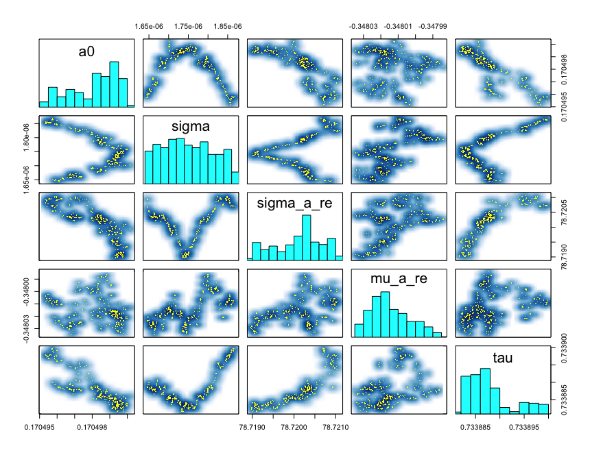
Here is the pairs-plot:
I tried also double of the iteartions from 1000 to 2000… the traceplots didn’t really change to lower iterations.
Btw, i also get these warning messages:
Warning messages:
1: There were 2000 transitions after warmup that exceeded the maximum treedepth. Increase max_treedepth above 10. See
Runtime warnings and convergence problems
2: There were 2 chains where the estimated Bayesian Fraction of Missing Information was low. See
Runtime warnings and convergence problems
3: Examine the pairs() plot to diagnose sampling problems
I’ll now try the seed-thing…
Thanks very much in advance,
Annika
My honest suggestion is to post the model if you can, the community will help you pinpoint the problem in your model. Without model it is hard to know what is going on.
i made another topic about my model, so i didn’t want to spam. I’m so sorry if i do. If there are any problems with my two different topics let me know, maybe i can put them together then…
But actually the model code in the other topic is slightly different. So here is my model code:
data {
 int<lower=0> Ni;            // Number of observations (an integer)
 int<lower=0> Nj;            // Number of clusters (an integer)
 int<lower=1> cluster[Ni];   // Cluster IDs
 vector[Ni] Y;               // output
 vector[Ni] X;               // X as in intervalls
 matrix[Nj, Ni] B;           // splines-matrix

 }


parameters {
  row_vector[Nj] a_raw;          //rows of the b-splines
  real a0;                       //slope ??
  real<lower=0> sigma;           //std.dev.
  real<lower=0> tau;             //coeff of b-splines
  vector[Ni] a_re;               //varying intercepts
  real mu_a_re;
  real<lower=0,upper=100> sigma_a_re;
}

transformed parameters  {
  row_vector[Nj] a;
  vector[Ni] Y_hat_sp;
  vector[Ni] Y_hat_re;

  a = a_raw*tau;

  for (i in 1:Ni){
    Y_hat_re[i] = a_re[cluster[i]];     //random effects
  }
    Y_hat_sp =  a0*X + to_vector(a*B);   // linear model and splines


 }

 model {

  sigma_a_re ~ uniform(0, 100);         //random effects sigma
  a_re ~ normal(mu_a_re, sigma_a_re);   //random effects distribution

  a_raw ~ normal(0, 1);                 //splines
  tau ~ normal(0, 1);                   //splines coeff distribution

  sigma ~ uniform(0, 100);              //model sigma

  for (i in 1:Ni)
  Y ~ normal(Y_hat_re + Y_hat_sp, sigma); //model


}
Thank you very much!
In the last part of your stan code, I find that you forget [i] .
In model block, sigma moves in range [0,100] .
On the other hand, in parameter block, its range is [0, \infty], so, I add upper=1 for a parameter sigma
I cannot remove non-convergent issues but, it looks better to modify your codes about the above two points.
.
Modified Stan file
   data {
     int<lower=0> Ni;            // Number of observations (an integer)
     int<lower=0> Nj;            // Number of clusters (an integer)
     int<lower=1> cluster[Ni];   // Cluster IDs
     vector[Ni] Y;               // output
     vector[Ni] X;               // X as in intervalls
     matrix[Nj, Ni] B;           // splines-matrix

     }


    parameters {
      row_vector[Nj] a_raw;          //rows of the b-splines
      real a0;                       //slope ??
      real<lower=0,upper=1> sigma;           //std.dev.
      real<lower=0> tau;             //coeff of b-splines
      vector[Ni] a_re;               //varying intercepts
      real mu_a_re;
      real<lower=0,upper=100> sigma_a_re;
    }

    transformed parameters  {
      row_vector[Nj] a;
      vector[Ni] Y_hat_sp;
      vector[Ni] Y_hat_re;

      a = a_raw*tau;

      for (i in 1:Ni){
        Y_hat_re[i] = a_re[cluster[i]];     //random effects
      }
        Y_hat_sp =  a0*X + to_vector(a*B);   // linear model and splines


     }

     model {

      sigma_a_re ~ uniform(0, 100);         //random effects sigma
      a_re ~ normal(mu_a_re, sigma_a_re);   //random effects distribution

      a_raw ~ normal(0, 1);                 //splines
      tau ~ normal(0, 1);                   //splines coeff distribution

      sigma ~ uniform(0, 100);              //model sigma

      for (i in 1:Ni)
      Y[i] ~ normal(Y_hat_re[i] + Y_hat_sp[i], sigma); //model


    }
R code
Ni <- 10L
   Nj <-3L
   cluster <-1:10
  Y <-runif(10)
   X <- runif(10)
   B <- matrix(1:30, nrow=3, ncol=10)


   dat <- list(
 Ni  =Ni,
 Nj   =Nj,
 cluster  =cluster,
 Y  =Y,
 X =X,
 B  =B

   )
   model  <- rstan::stan_model("a.stan")

   fit <- rstan::sampling(model,data=dat, chains =3 )
traceplot(fit)Unfortunately with my simulated data the traceplots still stay the same…
here is how i simulated my data:
#Splines
set.seed(123)
X1 <- seq(from=-5, to=5, length=150) # generating inputs
B2<- t(bSpline(X1, knots=seq(-4.9,5,1), degree=3, intercept = TRUE)) # creating the B-splines
num_data <- length(X1)
num_basis <- nrow(B2)
a0 <- 0.2 # slope
a <- rnorm(num_basis, 0, 1) # coefficients of B-splines

#Random Effects
set.seed(123)
sigma_u0 <- 1
u_0j     <- rnorm(num_basis, mean = 0, sd = sigma_u0) # "Random intercepts"
beta_0j  <- rep(u_0j, length=num_data) # Varying intercepts
cluster  <- rep(1:num_basis, length=num_data) # Cluster indicator
Y_true2 <- beta_0j + as.vector(a0*X1 + a%*%B2)   # generating the output -> multiplication of intercept w/ X plus matrix multiplication of a and B (Splines)


# Combine
dat      <- list(Ni      = num_data,
                 Nj      = num_basis,
                 cluster = cluster,
                 Y       = Y_true2,
                 X       = X1,
                 B       = B2
)
Realy !? I tried with your data again, then R hat looks good.
Inference for Stan model: a.
3 chains, each with iter=2000; warmup=1000; thin=1;
post-warmup draws per chain=1000, total post-warmup draws=3000.

              mean se_mean   sd  2.5%   25%   50%   75% 97.5% n_eff Rhat
a_raw[1]     -0.05    0.05 0.85 -1.84 -0.59 -0.05  0.59  1.48   292 1.02
a_raw[2]     -0.12    0.05 0.86 -1.78 -0.65 -0.18  0.42  1.57   331 1.01
a_raw[3]     -0.17    0.06 0.88 -2.28 -0.76 -0.08  0.40  1.50   198 1.02
a0            0.47    0.02 0.42 -0.40  0.23  0.47  0.70  1.38   368 1.02
sigma         0.27    0.01 0.14  0.06  0.17  0.25  0.34  0.59   284 1.02
tau           0.06    0.01 0.07  0.00  0.01  0.04  0.10  0.22    55 1.08
a_re[1]       0.46    0.02 0.30 -0.18  0.30  0.46  0.63  1.03   233 1.01
a_re[2]       0.11    0.03 0.39 -0.63 -0.16  0.13  0.31  0.96   134 1.02
a_re[3]       0.36    0.03 0.32 -0.30  0.17  0.38  0.55  1.01   133 1.03
a_re[4]       0.24    0.03 0.30 -0.41  0.06  0.24  0.40  0.87   141 1.02
a_re[5]       0.23    0.03 0.33 -0.42  0.04  0.23  0.39  0.93   160 1.01
a_re[6]       0.22    0.03 0.32 -0.40  0.02  0.21  0.40  0.88   155 1.02
a_re[7]       0.28    0.03 0.37 -0.45  0.06  0.28  0.47  1.16   115 1.02
a_re[8]       0.14    0.04 0.40 -0.66 -0.10  0.18  0.39  0.94   123 1.03
a_re[9]       0.43    0.04 0.44 -0.44  0.15  0.44  0.68  1.31   115 1.02
a_re[10]      0.23    0.03 0.38 -0.50  0.01  0.22  0.44  1.10   163 1.02
mu_a_re       0.26    0.03 0.31 -0.38  0.08  0.28  0.42  0.92   120 1.03
sigma_a_re    0.25    0.01 0.16  0.04  0.15  0.22  0.32  0.68   162 1.01
a[1]          0.01    0.01 0.07 -0.10 -0.02  0.00  0.02  0.17   102 1.05
a[2]          0.00    0.01 0.08 -0.20 -0.03  0.00  0.01  0.20    79 1.04
a[3]         -0.01    0.01 0.10 -0.22 -0.02  0.00  0.01  0.12    64 1.06
Y_hat_sp[1]   0.08    0.02 0.17 -0.35  0.02  0.11  0.18  0.36    97 1.03
Y_hat_sp[2]   0.34    0.03 0.37 -0.47  0.14  0.36  0.54  1.09   210 1.02
Y_hat_sp[3]   0.16    0.02 0.27 -0.53  0.03  0.18  0.32  0.68   144 1.02
Y_hat_sp[4]  -0.08    0.02 0.20 -0.62 -0.17 -0.06  0.03  0.26   101 1.02
Y_hat_sp[5]   0.03    0.02 0.26 -0.63 -0.09  0.03  0.18  0.52   118 1.02
Y_hat_sp[6]  -0.08    0.02 0.27 -0.74 -0.22 -0.06  0.08  0.39   119 1.02
Y_hat_sp[7]   0.05    0.03 0.35 -0.71 -0.13  0.05  0.27  0.73   134 1.02
Y_hat_sp[8]   0.11    0.03 0.42 -0.79 -0.12  0.10  0.37  0.94   145 1.02
Y_hat_sp[9]   0.20    0.04 0.51 -0.89 -0.08  0.19  0.52  1.21   161 1.02
Y_hat_sp[10] -0.22    0.03 0.41 -1.11 -0.46 -0.19  0.04  0.53   150 1.02
Y_hat_re[1]   0.46    0.02 0.30 -0.18  0.30  0.46  0.63  1.03   233 1.01
Y_hat_re[2]   0.11    0.03 0.39 -0.63 -0.16  0.13  0.31  0.96   134 1.02
Y_hat_re[3]   0.36    0.03 0.32 -0.30  0.17  0.38  0.55  1.01   133 1.03
Y_hat_re[4]   0.24    0.03 0.30 -0.41  0.06  0.24  0.40  0.87   141 1.02
Y_hat_re[5]   0.23    0.03 0.33 -0.42  0.04  0.23  0.39  0.93   160 1.01
Y_hat_re[6]   0.22    0.03 0.32 -0.40  0.02  0.21  0.40  0.88   155 1.02
Y_hat_re[7]   0.28    0.03 0.37 -0.45  0.06  0.28  0.47  1.16   115 1.02
Y_hat_re[8]   0.14    0.04 0.40 -0.66 -0.10  0.18  0.39  0.94   123 1.03
Y_hat_re[9]   0.43    0.04 0.44 -0.44  0.15  0.44  0.68  1.31   115 1.02
Y_hat_re[10]  0.23    0.03 0.38 -0.50  0.01  0.22  0.44  1.10   163 1.02
lp__         13.41    0.80 6.36  0.86  8.99 13.44 17.80 25.48    64 1.05

Samples were drawn using NUTS(diag_e) at Wed Aug 07 17:48:07 2019.
For each parameter, n_eff is a crude measure of effective sample size,
and Rhat is the potential scale reduction factor on split chains (at
convergence, Rhat=1).


check_hmc_diagnostics(fit)

Divergences:
599 of 3000 iterations ended with a divergence (19.9666666666667%).
Try increasing 'adapt_delta' to remove the divergences.

Tree depth:
0 of 3000 iterations saturated the maximum tree depth of 10.

Energy:
E-BFMI indicated no pathological behavior.
R scripts
    #Splines
    set.seed(123)
    X1 <- seq(from=-5, to=5, length=150) # generating inputs
    B2<- t(bSpline(X1, knots=seq(-4.9,5,1), degree=3, intercept = TRUE)) # creating the B-splines
    num_data <- length(X1)
    num_basis <- nrow(B2)
    a0 <- 0.2 # slope
    a <- rnorm(num_basis, 0, 1) # coefficients of B-splines

    #Random Effects
    set.seed(123)
    sigma_u0 <- 1
    u_0j     <- rnorm(num_basis, mean = 0, sd = sigma_u0) # "Random intercepts"
    beta_0j  <- rep(u_0j, length=num_data) # Varying intercepts
    cluster  <- rep(1:num_basis, length=num_data) # Cluster indicator
    Y_true2 <- beta_0j + as.vector(a0*X1 + a%*%B2)   # generating the output -> multiplication of intercept w/ X plus matrix multiplication of a and B (Splines)


    # Combine
    dat      <- list(Ni      = num_data,
                     Nj      = num_basis,
                     cluster = cluster,
                     Y       = Y_true2,
                     X       = X1,
                     B       = B2
    )


       model  <- rstan::stan_model("a.stan")

       fit <- rstan::sampling(model,data=dat, chains =3 )
       traceplot(fit)
Stan file named a.stan in the above R code
data {
 int<lower=0> Ni;            // Number of observations (an integer)
 int<lower=0> Nj;            // Number of clusters (an integer)
 int<lower=1> cluster[Ni];   // Cluster IDs
 vector[Ni] Y;               // output
 vector[Ni] X;               // X as in intervalls
 matrix[Nj, Ni] B;           // splines-matrix

 }


parameters {
  row_vector[Nj] a_raw;          //rows of the b-splines
  real a0;                       //slope ??
  real<lower=0,upper=1> sigma;           //std.dev.
  real<lower=0> tau;             //coeff of b-splines
  vector[Ni] a_re;               //varying intercepts
  real mu_a_re;
  real<lower=0,upper=100> sigma_a_re;
}

transformed parameters  {
  row_vector[Nj] a;
  vector[Ni] Y_hat_sp;
  vector[Ni] Y_hat_re;

  a = a_raw*tau;

  for (i in 1:Ni){
    Y_hat_re[i] = a_re[cluster[i]];     //random effects
  }
    Y_hat_sp =  a0*X + to_vector(a*B);   // linear model and splines


 }

 model {

  sigma_a_re ~ uniform(0, 100);         //random effects sigma
  a_re ~ normal(mu_a_re, sigma_a_re);   //random effects distribution

  a_raw ~ normal(0, 1);                 //splines
  tau ~ normal(0, 1);                   //splines coeff distribution

  sigma ~ uniform(0, 100);              //model sigma

  for (i in 1:Ni)Y[i] ~ normal(Y_hat_re[i] + Y_hat_sp[i], sigma); //model


}that’s crazy! i don’t know what’s going on with my computer/R/Rstan… :D i will close down R and open it again.
Please use my stan code.
a.stan) in your working directory.If you cannot get same one, then I will give up! :’-D
I don’t get it. It doesn’t work when i do it! Could it be that my stan version is too old or something? I absolutely don’t get it!
My rstan version is 2.19.2
I have the 2.18.2… i will update it, maybe this is the problem…?
I do not know., but if you remove and reinstall Rstan, then you should remove all tools related rstan.
If you remove only rstan, then it will cause installation error.
When I install stan, then I always remove all of R, and reinstall then.
Anyway Good Luck. Bye Bye.
Thank you so much for your help! I appreciate it.
Have a good day!
actually it seems like your stan code didn’t use my data, because a_raw is there just 3 times in your summary, and the other observations 10 times, as you simulated it before…? With my simulated data you should have 14x a_raw and the other observations 150 times.
and i think the point is, that you didn’t have the splines2 package installed and so it didn’t run the spline, and consequently it didn’t do the new Ni, Nj, and so on and so on…
You are correct!
I did not install spline2.
The convergent problem depends on data.
So, the stan file it self is correct for my data,
but for your data, it is something wrong.
I give up.
thank anyways! i will work on my data :)
Using your data X1 with length=26 instead length=150 , I get convergence.
If length is less than 26, then the model get a better convergence.
I am not sure the reason why model does not converge when the length is more greater.
I guess
if length is greater, then number of model parameter also increases,
On the other hand, almost all components of B2 is zero, so B2 does not contribute to estimates.
So lack of information gives non uniqueness of estimates and it causes the convergent issues.
Of course I do not know !!
length=26 is not so bad as following image;
length=150 is as following image;
library(splines2)

#Splines
set.seed(123)


# X1 <- seq(from=-5, to=5, length=150) # generating inputs
X1 <- seq(from=-5, to=5, length=26 ) # generating inputs

B2<- t(bSpline(X1, knots=seq(-4.9,5,1), degree=3, intercept = TRUE)) # creating the B-splines

num_data <- length(X1)
num_basis <- nrow(B2)
a0 <- 0.2 # slope
a <- rnorm(num_basis, 0, 1) # coefficients of B-splines


###################

knots <- c(-4.9,5,1)
bsMat <- bSpline(X1, knots=seq(-4.9,5,1), degree=3, intercept = TRUE)

library(graphics)
matplot( X1, bsMat, type = "l", ylab = "Piecewise constant B-spline bases")
abline(v = knots, lty = 2, col = "gray")
#########################


#Random Effects
set.seed(123)
sigma_u0 <- 1
u_0j     <- rnorm(num_basis, mean = 0, sd = sigma_u0) # "Random intercepts"
beta_0j  <- rep(u_0j, length=num_data) # Varying intercepts
cluster  <- rep(1:num_basis, length=num_data) # Cluster indicator
Y_true2 <- beta_0j + as.vector(a0*X1 + a%*%B2)   # generating the output -> multiplication of intercept w/ X plus matrix multiplication of a and B (Splines)


# Combine
dat      <- list(Ni      = num_data,
                 Nj      = num_basis,
                 cluster = cluster,
                 Y       = Y_true2,
                 X       = X1,
                 B       = B2,
                 Sparse  =10
                 # BB      = B3

)


 model  <- rstan::stan_model("a.stan")


fit <- rstan::sampling(model,data=dat, chains =3 ,seed =123456)
traceplot(fit)