Correlation of estimated SE with covariate leads to correlated parameters

Hi,
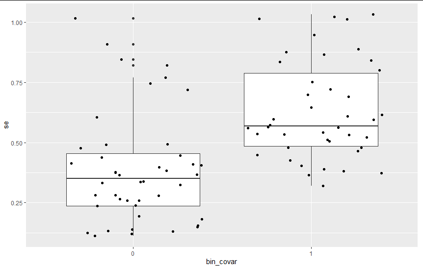
I eventually figured out that the correlation I was getting between my parameters of interest intercept and covar_effect was due to the fact that my binary covariate binary_covar is correlated with the se (higher SE for observations with binary_covar=1).
I’m a bit foggy on why that would lead to correlations in the posterior distributions, and also how bad that is, and also how I could fix it?
Thank you!

my model:

data{

  ///
	int <lower=1> N; // tot observed
	int <lower=1> Ngroup; // unique types of 
	
	vector[N] expvals;
	vector[N] se;
	vector[Ngroup] binary_covar;	
	int<lower=1, upper=Ngroup> group_id[N];	
  int<lower = 0, upper = 1> run_estimation; // a switch to evaluate the likelihood
  
}
parameters{
	vector[Ngroup] intercept_tilde;
	real covar_effect;
	real<lower=0> intercept_sd;
	real intercept;
}
transformed parameters{
	real Xeff_rep[N];

	vector[Ngroup] intercept_per_group;
	vector[Ngroup] group_mean;

	intercept_per_group = intercept_tilde * intercept_sd  + intercept; 
	group_mean = intercept_per_group + (binary_covar - mean(binary_covar) )* covar_effect; //+ ;
	
	for (i in 1:N){	
	     Xeff_rep[i] = group_mean[group_id[i]] ;
	  }
}

model {
      covar_effect ~ normal(0, .5); // 
      intercept ~ normal(0, .5); //
      intercept_sd ~ normal(0, .5); //normal(0, 1);
      intercept_tilde ~ std_normal(); //normal(0, 1);
      if(run_estimation==1){
         expvals ~ normal(Xeff_rep, se); // same as theta (transformed theta-tilde) in 8 schools
	    }
 }
 
generated quantities{
	  real eff_rep[N];
	  for (ix in 1:N){
	      eff_rep[ix] = normal_rng(group_mean[group_id[ix]], se[ix]);
	  }
}

Some data:

{"N":[86],"Ngroup":[43],"expvals":[-1.0914,-0.8639,-1.7732,-0.0152,-1.0071,-0.6503,-0.6973,-0.1273,-1.7947,0.3659,-1.1673,-0.5,-1.3925,-0.7708,-0.2552,-0.7064,-1.0336,-0.1527,-0.9017,-0.6918,-1.5845,-0.6171,0.2943,0.1781,0.2469,0.2767,0.1855,0.1515,0.3643,1.1286,0.4952,-0.1314,-0.4427,-0.2831,-1.3268,0.0577,0.4858,-0.3076,0.1341,-0.2223,1.1405,0.0301,0.4403,-1.0552,0.802,-0.2828,-0.9133,-1.3777,-0.1958,-1.1979,-0.7611,-1.2373,-0.9892,-0.3194,-1.6546,-0.5434,-0.4642,-0.5392,-0.6725,-0.3566,0.2213,-0.4259,-0.1281,-0.2893,-0.799,-0.3111,-0.0517,0.4879,0.145,0.1524,0.3558,0.2888,1.1802,0.1139,0.0591,0.4076,0.626,1.3808,-0.2103,0.5548,1.008,0.1728,-0.0534,0.562,0.2475,-1.7548],"se":[0.4788,0.7205,1.0145,0.5652,0.5604,0.4788,0.3721,0.8752,0.8874,0.6975,0.506,0.4642,0.3887,0.5622,0.493,0.5357,0.7515,0.5215,0.3197,0.865,0.609,0.5319,0.377,0.2579,0.1117,0.4388,0.2591,0.2365,0.1942,0.8206,0.1383,0.2816,0.4914,0.3641,0.6041,0.2807,0.4474,0.8455,0.125,0.406,0.339,0.1336,0.7699,0.4028,1.0223,1.0117,0.3652,0.5111,0.6161,0.4261,0.572,1.0315,0.8354,0.6461,0.5972,0.3807,0.6915,0.4103,0.5951,0.8004,0.5424,0.4479,0.9472,0.8415,0.5342,0.3658,0.3318,0.1209,0.4139,0.2654,0.2379,0.182,0.7462,0.1497,0.3245,0.4779,0.3838,0.7193,0.3368,0.374,1.0161,0.1316,0.3972,0.2785,0.1548,0.9091],"binary_covar":[0,0,0,1,1,1,1,0,1,0,1,1,1,0,1,0,1,0,0,0,1,0,0,1,1,0,1,0,0,0,0,1,1,1,0,1,0,0,1,0,1,1,0],"group_id":[4,5,6,7,11,9,12,13,15,17,21,24,25,27,30,32,33,34,36,39,41,42,1,2,3,8,10,14,16,18,19,20,22,23,26,28,29,31,35,37,38,40,43,4,5,6,7,11,9,12,13,15,17,21,24,25,27,30,32,33,34,36,39,41,42,1,2,3,8,10,14,16,18,19,20,22,23,26,28,29,31,35,37,38,40,43],"run_estimation":[1]} 


the correlation is 0.49

1 Like

Hi,
sorry for not getting to you earlier - did you manage to make some progress in the meantime?

Could you share a bit more of your reasoning? I don’t think I can follow why that could/should be the case.

In many cases correlation in the posterior arises because the data do not inform both parameters individually, but only tell us something about their sum/difference/other combination.

Also - is the correlation a problem? Are your model diagnostics bad? If not then maybe this is the correct posterior?

If you haven’t solved the issue yet, I’ll be glad to discuss it further!

Best of luck with your model!

Thanks for the reply! I did not figure that out via reasoning but by empirical results… if I replace the se vector in the input list with a constant SE ( input$se = rep(.5, length(input$se)) ) then re-run everything I get a different result with no correlations. But maybe it doesn’t matter since the marginal distributions look the same more or less? I guess that was part of my question, if it matters? I can’t think of why the true posterior would be correlated.

I don’t see anything obviously wrong with the diagnostics

Inference for Stan model: simp2.
4 chains, each with iter=5000; warmup=2000; thin=1; 
post-warmup draws per chain=3000, total post-warmup draws=12000.

              mean se_mean   sd  2.5%   25%   50%   75% 97.5% n_eff Rhat
intercept    -0.26       0 0.05 -0.35 -0.29 -0.26 -0.22 -0.16  8941    1
covar_effect -0.93       0 0.10 -1.13 -1.00 -0.94 -0.87 -0.73  8613    1

Thanks again!

1 Like

That’s an interesting check!

Looking a bit closer, I think what is happening is that you are not having enough data to learn all the structure you are imposing very well. Looking at an extended pairs plots:

(intercept_sd has been log-transformed)

You can noitce, that when intercept_sd is low (the varying intercept is allowed to explain only small part of the total variation), your intercept and covar_effect are relatively tightly determined. But when intercept_sd is large, they are allowed to take a much wider range of values.

This problem is seen even when setting all the .se to .5:

So what I think is going on is that due to the low number of repetitions per group, the varying intercepts are not well determined and can take in part of the influence attributable to covar_effect (since covar_effect is constant withng group).

Not completely sure why that leads to correlations with the varying SE and not with constant SE. One possibility is that this is linked to the fact that SE is correlated with the covariate (see figure below) - when I set the SE to be constant per binary_covar value, I also get the correlation. This might be further connected to the way you use centering of the binary covariate - if I don’t center I get a negative correlation between intercept and cover_effect, meaning that the data are consistent with either a larger intercept and small difference between covariate values (i.e. the intercept is closer to the overall mean) and with smaller intercept and larger difference between covariate value. Which is once again the situation where your data are unable to differentiate between the various contributions.

But I think the relationship between the intercept_sd and the fixed effects is the most interesting thing happening here.

Does that make sense?

1 Like

Sorry for the very delayed response. I am still dealing with this issue, though.

I had centered the binary_covar because of identifiability issues that led to the negative correlation between intercept and covar_effect, which was how I first started looking at the correlation between these variables.

The data that I was using to fit the model was actually sampled, from the same model, so there should not be any true correlation between those parameters. I tried implementing a simpler model (below) where I remove the per-group parameters and only try to learn intercept and covar_effect as if there were no groups, based on your hypothesis that it was too many intercepts (so now the binary_covar only applies to individual data points not groups), but the same correlation happens.

My workaround is to cut-off my input data and remove any of the input with a value for se that is below 0.3 or so. It’s kind of ugly!

Thanks, if you have any thoughts about how I could model this better or if I could pretend it’s not happening, I’d love to hear it.

data{

  ///
	int <lower=1> N; // tot observed
	vector[N] expvals;
	vector[N] se;
	vector[N] binary_covar;	
  int<lower = 0, upper = 1> run_estimation; // a switch to evaluate the likelihood
  
}
parameters{
	real covar_effect;
	real intercept;
}
transformed parameters{
	real Xeff_rep[N];

	for (i in 1:N){	
	     Xeff_rep[i] = intercept + (binary_covar[i] - mean(binary_covar) )* covar_effect;
	  }
}

model {
      covar_effect ~ normal(0, .5); // 
      intercept ~ normal(0, .5); //
 }

Unfortunately, I can’t really dig deeply in the model due to time constraints. There is a bunch of diagnostic techniques briefly mentioned at Divergent transitions - a primer, which could help you investigate further and gain some understanding. I would definitely try to simplify the model further to see when the problematic behaviour disappears.

I might be misunderstanding you here, but it seems you are conflating a correlation in the model (e.g. when two parameters are modelled as multivariate normal distrubted) and a correlation in the posterior, which can happen regardless of whethere the model (or more broadly the data generating process) has any correlations. I.e. you can easily have all sorts of weird structure (including correlations) in your posterior samples, even if your code to simulate the data perfectly matches the model and there are no correlations in the model. Understanding why this structure arises in the posterior is often the best way to diagnose and resolve issues - unfortunately there is no general way to do this, one needs to think hard about the model one sees.

Best of luck with the model!

1 Like

Understood, thanks for taking a look at it.

Unfortunately, i think it’s not possible to simplify the model more as it only has 2 parameters at this point and is still showing the strange behavior. I know what you’re saying about the difference between the model and the posterior. My model does not include any correlations between these but the posterior does, even in simulated data, which is the problem I was trying to solve. And yes, I found this problem by doing some of the diagnostics (though I don’t have any divergences).

No worries, thanks for your time.