Correcting for bad sampling the correct way

[dankehila]

Hi all

The observed outcome in my study is counts (specifically, bacterial counts), but the counts are distroted in an interesting way: some samples are older than others, making older samples have lots of bacteria (even if they started with a small amount) because there was time for them to grow exponentially. The people who collected the data could not stop some samples from getting old, but they could at least record the age of every sample, which gives me the opportunity to correct for this aging.

Briefly, for an initial bacterial sample i with count Y_{0}^{i}, the actual observed value after reaching age t_{i} is Y_{measured}^{i} = Y_{0}^{i} e^{r t_{i}}, where r is the growth rate of the bacteria, a parameter to be estimated. As is probably obvious to many of you, an initial count of 0 would stay 0, and our data does contain a lot of zeroes (~70%), but the non-zero portion would get stretched down the number line depending on how old every sample is.

Note that we’re interested in the values before the distortion due to growth: that is, I’m interested in modelling Y_{0}^{i} and estimate parameters (mean etc) for it, and not for the measured value, which is distorted. As such, I will need to estimate r as well. A statistical model based on Y_{0}^{i} following a poisson or negative binomial is fine, but we’re measuring Y_{measured}^{i} instead.

I have a feeling that doing the following is a statistical no no:

\frac{Y_{measured}^{i}}{e^{r t_{i}}} \sim \mathrel{NegBin(\mu,\phi)}

That is, dividing my outcome by the vector of expected growth due to age. But if in Stan I do this:

data{
int N;
vector[N] Ymeasured;
vector[N] t;
}
parameters{
vector[N] y0;
real<lower=0> r;
real<lower=0> phi;
...
}
transformed parameters{
vector[N] mu = y0*exp(r * t);
}
model{
Ymeasured ~ neg_binomial_2(mu,phi);
}

This is a problem too because Ymeasured itself is not expected to be distributed as a negative binomial, just because Y0 is, and even if it was, the overdispersion parameter phi would be different before and after aging.

I think if I change my model from a negative binomial to a poisson or a hurdle type, I will still have this same problem: after distortion, I’m not sure of the distribution anymore, but I have better ideas (and more interest in) the distribution of y0.

Any advice appreciated

[jsocolar]

@dankehila

I have a feeling that doing the following is a statistical no no:

\frac{Y_{measured}^{i}}{e^{r t_{i}}} \sim \mathrel{NegBin(\mu,\phi)}Yimeasurederti∼NegBin(μ,ϕ)

This doesn’t work because it results in passing non-integer outcomes to a negative binomial.

What to do here depends substantially on some aspects of the data generating process that are not clear. Suppose we observe a count Y_{old} corresponding to a sample that, when it was new, would have yielded a hypothetical count Y_{new}. Is Y_{old} an exhaustive count of all of the progeny descending from exactly the individuals represented in Y_{new}? Or is Y_{new} a Poisson sample from some underlying initial concentration C_{new} which then grows exponentially to become C_{old} from which we draw a new Poisson sample Y_{old}? Or something else?

In other words, if there is any sampling variation in the hypothetical Y_{old}, is that sampling variation pushed forward through the exponential growth process? Or does the exponential growth occur in some mean-field background that gets represented by a concentration and then sampled (presumably Poisson) to yield the counts? Note that in this latter case, the counts Y_{old} might still be negative binomial rather than Poisson, i.e. if there is gamma-distributed process variation in the concentrations followed by Poisson-distributed sampling variation in the counts.

[dankehila]

Before aging, the sample Y_{new} is a vector of observed samples, likely taken from an overdispersed (negbin) count distribution. I believe the Y_{new} are negbin distributed because, if I subset the observations to only the samples which were measured when still quite fresh (new), I can presumably see the distribution of Y_{new} before the distortion due to old age. In this fresh sample subset, the data fits a negbin well, and far better than a poisson, mostly because there are both zeroes and large numbers.

Then, what sample age does is it takes the negative binomial Y_{new} and pushes the non zero values further forward, like you said. I am not exactly sure I understand the mean-field scenario, but hope that what I provide here clarifies the situation.

(
On a further note, because of overdispersion I also checked if a zero-inflated poisson or zero-inflated negative binomial seem to fit the fresh data subset better than negbin by itself, but I couldn’t find evidence that it fits it any better than the standard negative binomial. To compare fits I used posterior prediction plots as well as standard R package heuristics like chisq, information criteria and quantile plots, so maybe it’s not the most thorough check, but it didn’t seem like there is a noticeable improvement to adding the complex zero-inflated feature so I was inclined to leave it as negbin for now (at least until I figure out how to correct for age and use the full dataset).
)

[jsocolar]

@dankehila

I am not exactly sure I understand the mean-field scenario, but hope that what I provide here clarifies the situation.

I think this is absolutely crucial to nail down, so I’ll try to be as specific as I can. Here are two scenarios (and bear in mind that other scenarios are possible as well). Does your situation correspond exactly to either of these two scenarios? Suppose you have an experimental replicate consisting of bacteria suspended in an aqueous medium. Suppose the samples are “fresh” at time t_1 and “stale” at time t_2.

Scenario 1: To estimate the number of bacteria in the replicate, you take a small aliquot at t_1. In the event of a fresh sample, you individually count all of the N bacteria (e.g. by plating on agar and counting colonies) immediately at t_1. In the event of a stale sample, you still take the aliquot at time t_1, and exponential growth happens only within the aliquot. That is, the aging process happens after the small aliquot has been taken.

Scenario 2: In the event of a stale sample, you wait until time t_2 to take the aliquot. Thus, the aging process happens within the larger experimental replicate before the small aliquot gets taken.

These scenarios are quite different for a number of reasons. For example, in scenario 1, the number of bacteria that you expect in a stale sample depends crucially on the discrete (presumably Poisson) sampling process that yielded the count when the sample was fresh. Also, in scenario 1 the number of bacteria in the growing population starts so small that you likely need to worry about the stochastic vagaries of growth rates in tiny populations of cells, whereas in scenario 2 you can expect the concentration to change smoothly and deterministically as the bacteria grow.

[dankehila]

Ah, now I understand much better, thank you. Scenario 2 is the case here.

Here’s exactly what’s happening:

Basically, fresh samples at t_{1} are all driven to the lab with a courier, and they arrive at time t_{2}, which is random for every sample: sometimes the courier does a fast job, sometimes the truck is held back for whatever reason.

Once it arrives at the lab a plating test is immediately performed

The date and time is recorded at sampling (t_{1}) and when it arrives at the lab for immediate testing (t_{2}), so we can get the age of the sample as the difference between the two.

The samples themselves are a very large volume and all the growth happens within them. The bacterial counting test measures the density of bugs in the larger sample.

[jsocolar]

I was hoping you’d say that, because it makes things dramatically easier. Recall that the negative binomial distribution can also be expressed as a gamma-poisson mixture. Since the removal of the aliquot is almost by definition a Poisson sampling process, the negative binomial distribution of the t_1 counts suggests that the distribution of the underlying concentrations is gamma. So we can write the t_1 model as:

C_i \sim \textrm{gamma}(a, b),
Y_i \sim \textrm{Poisson}(C_i)
where a and b are fitted parameters, and C is in units of (expected) bacteria per aliquot volume.

Now updating the model for a later timestep is straightforward:
Y_i \sim \textrm{Poisson}(e^{rt_i}C_i)

Moreover if C is gamma distributed, then \alpha C is also gamma-distributed, and in particular e^{rt_i}C_i is gamma distributed. Thus, Y_i is still negative binomial, and we can readily integrate out C, yielding an integrated sampling distribution for Y drawn from a negative binomial that depends on e^{rt_i} and the Gamma parameters a and b. How exactly to combine these quantities to yield the negative binomial parameters depends on what parameterization of the negative binomial you’re using. Unfortunately, I don’t have time right now to remember how Stan parameterizes and how to derive the appropriate terms, but the relationships given by Wikipedia should be enough to work it out: Negative binomial distribution - Wikipedia (coupled with the formula for the Gamma distribution that yields a scaling of some other Gamma; see Probability Density Function of Scaled Gamma Random Variable - Mathematics Stack Exchange).

Edit: a final point to make here is that even if you desire to model growth relationships more flexible than exponential (e.g. maybe some of these samples grow past the log phase and a sigmoidal relationship is more appropriate), you can still write this down easily by treating the parameters C_i explicitly. The sampling distribution for Y_i will no longer be negative binomial, because conditional on t_i, f(C_i, t_i) will no longer be gamma distributed if the function f is more complicated than a scalar multiple of C_i (after conditioning on t_i). So it won’t be easy to integrate out C_i. But you can still write the likelihood in terms of a latent parameter C_i by explicitly treating C_i as gamma, then computing f(C_i, t_i) as a transformed parameter, and then sampling the data from a Poisson parameterized by f(C_i, t_i).

[LucC]

Hi, another count model enthousiast here. I agree with the reasoning by @jsocolar, except perhaps for one point (which maybe I misunderstand):

@jsocolar

you can still write this down easily by treating the parameters C_iCiC_i explicitly. The sampling distribution for Y_iYiY_i will no longer be negative binomial

The conditional distribution of Y_i, given the expected density initial bacterial density per sampled volume \mu_{0i}, multiplication factor e^{rt_i}, and shape a, is still a negative binomial distribution. The only assumption is that the overdispersion of the bacterial counts is the same for all bacterial densities, which is probably fine (as long as each examined sample has the same volume). Stan has a negative binomial distribution that is parameterised in terms of its mean (or the log of the mean) and shape (called Phi in Stan). Your linear predictor for this would therefor be:

log(\mu_i) = rt_i + \mu_{0i} +...

And

Y_i ~ NB(\mu_i,a)

[jsocolar]

@LucC no disagreement here :)

The scenario I was referring to where Y_i would no longer be negative binomial is in the generalized case (not mentioned by the OP) where the growth function is not exponential, so that the ending concentration is no longer a scalar multiple of the starting concentration. In this case the ending concentration won’t be Gamma anymore, and mixing this new distribution with a Poisson won’t yield a negative binomial.

See

@jsocolar

Moreover if CCC is gamma distributed, then \alpha CαC\alpha C is also gamma-distributed, and in particular e^{rt_i}C_iertiCie^{rt_i}C_i is gamma distributed. Thus, Y_iYiY_i is still negative binomial, and we can readily integrate out CCC, yielding an integrated sampling distribution for YYY drawn from a negative binomial that depends on e^{rt_i}ertie^{rt_i} and the Gamma parameters aaa and bbb.

But then

@jsocolar

Edit: a final point to make here is that even if you desire to model growth relationships more flexible than exponential (e.g. maybe some of these samples grow past the log phase and a sigmoidal relationship is more appropriate), you can still write this down easily by treating the parameters C_iCiC_i explicitly. The sampling distribution for Y_iYiY_i will no longer be negative binomial

[dankehila]

Thank you @jsocolar for the wonderful solution.

@LucC , I think what Jacob was referring to was in case when the growth of the bacteria is not simply exponential, but for example, logistic. In the case of logistic growth, thee would be a maximum count which right-censors all growth. Then, the resulting distribution would not be a negative binomial.

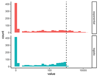
Here is some simulated data to show what I mean (and what I think Jacob meant) visually. The dashed line shows the maximum density (carrying capacity)

library(tidyverse);library(fitdistrplus)
phi = 0.1 #negative binomial shape parameter
mu = 30; # negative binomial mean
rt = 3; # growth term, assumed fixed for all Y for simplicity and visualization
Kap = 1e3; #maximum density for logistic growth
C = rgamma(1e3,phi,phi/mu) #calculating theta
pois_y = rpois(1e3,C)

#parameters are obtained as expected from poisson gamma mixture
fitdistrplus::fitdist(pois_y,'nbinom')

#applying growth to samples
pois_y_grown = rpois(1e3,C*exp(rt))  # exponential growth
pois_y_grown_logistic = rpois(1e3,C*Kap*exp(rt)/(Kap + C*(exp(rt)-1))) # logistic gorwth

# distribution fitting
# the new mean of pois_y_grown should be mu * exp(rt)
fitdistrplus::fitdist(pois_y_grown,'nbinom')
mu*exp(rt) # should be equal to new mean above

# this should not be the same if many samples reach the maximal density
fitdistrplus::fitdist(pois_y_grown_logistic,'nbinom')

# figure
tibble(exponential=pois_y_grown,logistic=pois_y_grown_logistic) %>% gather %>% 
  ggplot(aes(value,fill=key)) + geom_histogram(show.legend = F) + 
  scale_x_continuous(trans=scales::pseudo_log_trans(),breaks=c(0,100,10000)) + theme_classic()+
  labs(color = 'growth') + geom_vline(xintercept=Kap,linetype='dashed') + facet_grid(key~.)

Logistic growth may be possible to model in this case using a model with censoring. But for my purposes, it was obvious that bacteria could grow much more than they have even in the most dense samples, so I left it at exponential.

[LucC]

@jsocolar, I think I understood what you said, but failed to formulate my point as I actually meant it: I think that even in the case of non-exponential growth, the distribution of Y_i is negative binomial, conditional in the initial bacterial density \mu_{0i}, the multiplication factor f(t_i, \theta_i) (where \theta are the parameters of the non-exponential growht function), and shape a. The linear predictor then becomes:

log(\mu_i) = log(f(t_i, \theta_i)) + \mu_{0i} + ...

and still

Y_i ~ NB(\mu_i, a)

I don’t quite follow why a NB would not apply. Likewise, in your reasoning about the gamma-poisson mixture, given data t_i and conditional on growth function parameters \theta, f(t_i, \theta)C is still gamma-distributed.

[LucC]

@dankehila

@LucC , I think what Jacob was referring to was in case when the growth of the bacteria is not simply exponential, but for example, logistic. In the case of logistic growth, thee would be a maximum count which right-censors all growth.

I don’t think I agree (just yet). Even if the growth is logistic, that process only applies to the “true” bacterial density. The count Y_i that one observes in a sample volume is still subject to negative binomial (or Poisson if there is no clumping of bacteria) variation!

[LucC]

Maybe I am thinking of a different kind of “bacterial sample” here than the OP. I am thinking of a sample volume of growth medium from a larger specimen (e.g., a flask in which the bacteria grow), and the bacteria in that sample are counted (Y_i).

In your original post, you raise that the overdispersion phi would change if samples are older. If this is because the clumping of bacteria matters less and less as you get more bacteria in your sample, than you should fit a distributional model, where phi is a function of the true bacterial density \mu_i. I imagine that this function would be linear, just as in the case where phi scales up proportionally when you count larger sample volumes (the distribution of two identically NB-distributed variables is NB(2mu,2phi).

[EDIT: my reasoning assumes that scenario 2 applies, i.e., each aliquot i was sampled and enumerated at time t_i]

[jsocolar]

@LucC I think we’re all on the same page about the sampling scheme. Where we differ is that I’m imagining that the initial true density is gamma distributed, and the sampling variation around that density is Poisson (e.g. because we thoroughly mix the samples before taking the aliquot). So the negative binomial arises from Poisson sampling variation mixed via Gamma process variation.

You’re imagining that the initial density is fixed and the sampling variation negative binomial.

In my version, non-multiplicative growth morphs the process variation at time i into something that isn’t Gamma, and then I assume that sampling variation is still Poisson. The Poisson mixed by something that isn’t gamma yields something that isn’t negative binomial.

[LucC]

Ha! That’s an interesting difference of views indeed; it all depends on what we take the gamma mixture to represent. Thanks for clarifying your point of departure; fair point about mixing the samples before taking an aliqout (that’s a lot harder/impossible when you count parasite eggs in poo, which is what I typically model XD). Would you agree though that our two views lead to phenomologically the same distribution of a single observation Y_i? It’s just that when I say this observation Y_i is NB-distributed, and you say it isn’t, in our minds we must be conditioning on different parameters, right?

EDIT: moment of realisation (sorry if this is obvious to you, but this helped my thinking): the difference in our views is that if I were to take a second aliquot and count bacteria in it, in my view, I would redraw from the gamma mixture distribution, but you wouldn’t as you assume that the concentration in the second aliquot is exactly the same as in the first.