For the purpose of reporting an analysis we have run a normal hierarchical model and a few additional models as robustness checks (t-distributed error term, t-distributed priors for the random effects and a Tweedie distribution based model) and are inclined to go with the “conventional” one (linear hierarchical random effects model), as it seems to generate good fit - would you find this approach appropriate? Alternatively, would you suggest reporting results based on the t-distribution? Or the Tweedie Distribution? All of these models yield similar results/ fits.
The “conventional” model is a linear hierarchical random effects model with three layers along the following lines
model <- brm(DV ~ control1 + control 2 + (1 | Level_1) + (1|Level_1:Level_2) +(1|Level_1:Level_2:Level_3))
see the STAN code below:
functions {
}

data {

int<lower=1> N; // total number of observations

vector[N] Y; // response variable

int<lower=1> K; // number of population-level effects

matrix[N, K] X; // population-level design matrix

// data for group-level effects of ID 1

int<lower=1> N_1; // number of grouping levels

int<lower=1> M_1; // number of coefficients per level

int<lower=1> J_1[N]; // grouping indicator per observation

// group-level predictor values

vector[N] Z_1_1;

// data for group-level effects of ID 2

int<lower=1> N_2; // number of grouping levels

int<lower=1> M_2; // number of coefficients per level

int<lower=1> J_2[N]; // grouping indicator per observation

// group-level predictor values

vector[N] Z_2_1;

// data for group-level effects of ID 3

int<lower=1> N_3; // number of grouping levels

int<lower=1> M_3; // number of coefficients per level

int<lower=1> J_3[N]; // grouping indicator per observation

// group-level predictor values

vector[N] Z_3_1;

// data for group-level effects of ID 4

int<lower=1> N_4; // number of grouping levels

int<lower=1> M_4; // number of coefficients per level

int<lower=1> J_4[N]; // grouping indicator per observation

// group-level predictor values

vector[N] Z_4_1;

int prior_only; // should the likelihood be ignored?

}

transformed data {

int Kc = K - 1;

matrix[N, Kc] Xc; // centered version of X without an intercept

vector[Kc] means_X; // column means of X before centering

for (i in 2:K) {

means_X[i - 1] = mean(X[, i]);

Xc[, i - 1] = X[, i] - means_X[i - 1];

}

}

parameters {

vector[Kc] b; // population-level effects

real Intercept; // temporary intercept for centered predictors

real<lower=0> sigma; // dispersion parameter

vector<lower=0>[M_1] sd_1; // group-level standard deviations

vector[N_1] z_1[M_1]; // standardized group-level effects

vector<lower=0>[M_2] sd_2; // group-level standard deviations

vector[N_2] z_2[M_2]; // standardized group-level effects

vector<lower=0>[M_3] sd_3; // group-level standard deviations

vector[N_3] z_3[M_3]; // standardized group-level effects

vector<lower=0>[M_4] sd_4; // group-level standard deviations

vector[N_4] z_4[M_4]; // standardized group-level effects

}

transformed parameters {

vector[N_1] r_1_1; // actual group-level effects

vector[N_2] r_2_1; // actual group-level effects

vector[N_3] r_3_1; // actual group-level effects

vector[N_4] r_4_1; // actual group-level effects

real lprior = 0; // prior contributions to the log posterior

r_1_1 = (sd_1[1] * (z_1[1]));

r_2_1 = (sd_2[1] * (z_2[1]));

r_3_1 = (sd_3[1] * (z_3[1]));

r_4_1 = (sd_4[1] * (z_4[1]));

lprior += student_t_lpdf(Intercept | 3, 0, 2.5);

}

model {

// likelihood including constants

if (!prior_only) {

// initialize linear predictor term

vector[N] mu = rep_vector(0.0, N);

mu += Intercept;

for (n in 1:N) {
// add more terms to the linear predictor
mu[n] += r_1_1[J_1[n]] * Z_1_1[n] + r_2_1[J_2[n]] * Z_2_1[n] + r_3_1[J_3[n]] * Z_3_1[n] + r_4_1[J_4[n]] * Z_4_1[n];
}

target += normal_id_glm_lpdf(Y | Xc, mu, b, sigma);
}
// priors including constants

target += lprior;

target += std_normal_lpdf(z_1[1]);

target += std_normal_lpdf(z_2[1]);

target += std_normal_lpdf(z_3[1]);

target += std_normal_lpdf(z_4[1]);
}
generated quantities {

// actual population-level intercept

real b_Intercept = Intercept - dot_product(means_X, b);

}
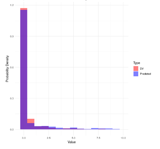
The DV and control variables of our hierarchical model are continuous.
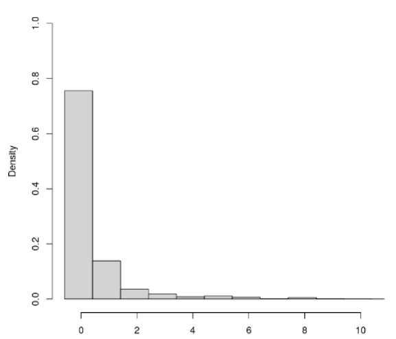
The distribution of the DV looks as follows:
This is a variance decomposition analysis. The effects of interest are the variance components of the three nested hierarchical levels.
The control control variable has a similar right skewed shape.
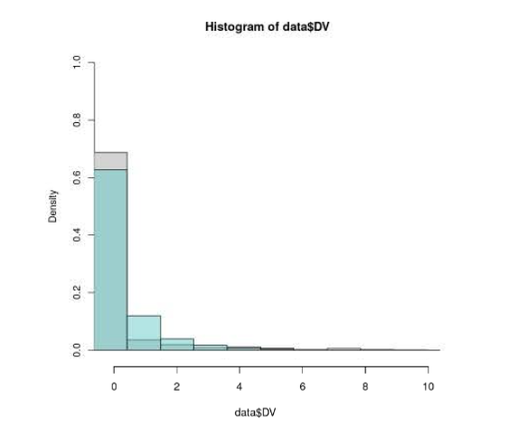
The predicted posterior (turkoise in the figure below) seems to fit reasonably well with the actual distribution of the DV(gray in the below figure) (the histogram is cut off on the right to zoom in more here).
The results of our conventional (linear hierarchical) model are as follows (the alternative models have similar results):
- Variance explained level 1: 2.9
- Variance explained level 2: 5.1
- Variance explained level 3: 5.3
- Variance explained control variable: 0.9
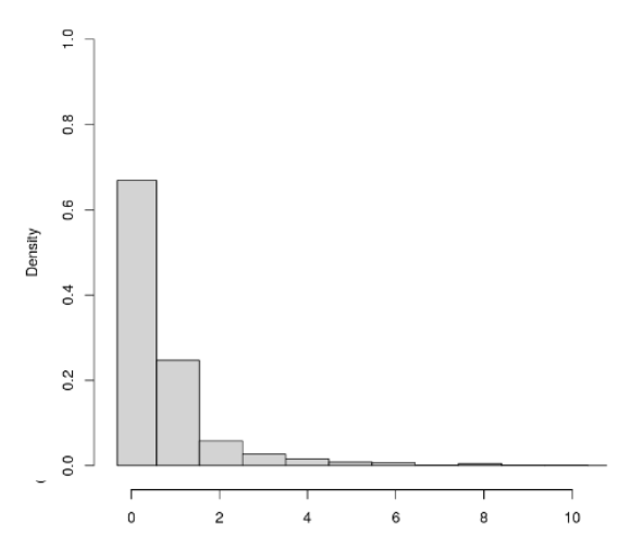
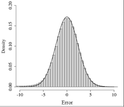
The distribution of the error term (posterior of DV - DV) looks as follows:
R heat for all variables is between 1.000 and 1.003 Effective samples size is > 1000 for every variable.
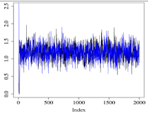
The normal model seems to converge well after some initial period (warm up is 2000 and sampling is 2000). Below, two markov chains after the warm up are shown (we ran 4 chains but the image is difficult to read with 4 chains).
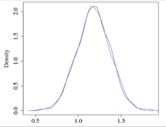
Another view of the distribution of two markov chains:
We also ran the model with t-distributed priors for the random effects, with t-distributed errors and with random effects that can vary for each level of the hierarchy and obtained similar results.
The estimates for the variance components that we obtain stay roughly the same.
Finally running a model with a Tweedie link function gives similar results for the variance components (see my other post here).
The details of the Tweedie model we ran can be found here. Note that the Tweedie model linked in here allows the random effects for each level to be drawn from different standard deviations. The convergence of the Tweedie model and its posterior also look good and we can provide them if this is helpful.
Finally, we noticed that the confidence intervals of the variance estimates of all models seem to be much wider than the confidence intervals of point estimates and asked in a post in this forum, whether this is normal and to be expected.
The posterior predicted DV vs actual DV for the Tweedie model looks as follows.