We are conducting a variance decomposition using a hierarchical linear random effects Bayesian model to investigate the variance in a DV that is affected by three nested layers. The DV is right skewed and we suspect that this is partly due to latent differences in the individuals. Because all the hierarchical factors are on the aggregate levels, we include a control variable for these individual differences, which leads to a well-fitting model in terms of the posterior of the DV. Is this a good approach?
I think you need to tell more about your model, inference diagnostics, and model checking diagnostics used
For the purpose of reporting an analysis we have run a normal hierarchical model and a few additional models as robustness checks (t-distributed error term, t-distributed priors for the random effects and a Tweedie distribution based model) and are inclined to go with the “conventional” one (linear hierarchical random effects model), as it seems to generate good fit - would you find this approach appropriate? Alternatively, would you suggest reporting results based on the t-distribution? Or the Tweedie Distribution? All of these models yield similar results/ fits.
The “conventional” model is a linear hierarchical random effects model with three layers along the following lines
model <- brm(DV ~ control1 + control 2 + (1 | Level_1) + (1|Level_1:Level_2) +(1|Level_1:Level_2:Level_3))
see the STAN code below:
functions {
}

data {

int<lower=1> N; // total number of observations

vector[N] Y; // response variable

int<lower=1> K; // number of population-level effects

matrix[N, K] X; // population-level design matrix

// data for group-level effects of ID 1

int<lower=1> N_1; // number of grouping levels

int<lower=1> M_1; // number of coefficients per level

int<lower=1> J_1[N]; // grouping indicator per observation

// group-level predictor values

vector[N] Z_1_1;

// data for group-level effects of ID 2

int<lower=1> N_2; // number of grouping levels

int<lower=1> M_2; // number of coefficients per level

int<lower=1> J_2[N]; // grouping indicator per observation

// group-level predictor values

vector[N] Z_2_1;

// data for group-level effects of ID 3

int<lower=1> N_3; // number of grouping levels

int<lower=1> M_3; // number of coefficients per level

int<lower=1> J_3[N]; // grouping indicator per observation

// group-level predictor values

vector[N] Z_3_1;

// data for group-level effects of ID 4

int<lower=1> N_4; // number of grouping levels

int<lower=1> M_4; // number of coefficients per level

int<lower=1> J_4[N]; // grouping indicator per observation

// group-level predictor values

vector[N] Z_4_1;

int prior_only; // should the likelihood be ignored?

}

transformed data {

int Kc = K - 1;

matrix[N, Kc] Xc; // centered version of X without an intercept

vector[Kc] means_X; // column means of X before centering

for (i in 2:K) {

means_X[i - 1] = mean(X[, i]);

Xc[, i - 1] = X[, i] - means_X[i - 1];

}

}

parameters {

vector[Kc] b; // population-level effects

real Intercept; // temporary intercept for centered predictors

real<lower=0> sigma; // dispersion parameter

vector<lower=0>[M_1] sd_1; // group-level standard deviations

vector[N_1] z_1[M_1]; // standardized group-level effects

vector<lower=0>[M_2] sd_2; // group-level standard deviations

vector[N_2] z_2[M_2]; // standardized group-level effects

vector<lower=0>[M_3] sd_3; // group-level standard deviations

vector[N_3] z_3[M_3]; // standardized group-level effects

vector<lower=0>[M_4] sd_4; // group-level standard deviations

vector[N_4] z_4[M_4]; // standardized group-level effects

}

transformed parameters {

vector[N_1] r_1_1; // actual group-level effects

vector[N_2] r_2_1; // actual group-level effects

vector[N_3] r_3_1; // actual group-level effects

vector[N_4] r_4_1; // actual group-level effects

real lprior = 0; // prior contributions to the log posterior

r_1_1 = (sd_1[1] * (z_1[1]));

r_2_1 = (sd_2[1] * (z_2[1]));

r_3_1 = (sd_3[1] * (z_3[1]));

r_4_1 = (sd_4[1] * (z_4[1]));

lprior += student_t_lpdf(Intercept | 3, 0, 2.5);

}

model {

// likelihood including constants

if (!prior_only) {

// initialize linear predictor term

vector[N] mu = rep_vector(0.0, N);

mu += Intercept;

for (n in 1:N) {
// add more terms to the linear predictor
mu[n] += r_1_1[J_1[n]] * Z_1_1[n] + r_2_1[J_2[n]] * Z_2_1[n] + r_3_1[J_3[n]] * Z_3_1[n] + r_4_1[J_4[n]] * Z_4_1[n];
}

target += normal_id_glm_lpdf(Y | Xc, mu, b, sigma);
}
// priors including constants

target += lprior;

target += std_normal_lpdf(z_1[1]);

target += std_normal_lpdf(z_2[1]);

target += std_normal_lpdf(z_3[1]);

target += std_normal_lpdf(z_4[1]);
}
generated quantities {

// actual population-level intercept

real b_Intercept = Intercept - dot_product(means_X, b);

}
The DV and control variables of our hierarchical model are continuous.
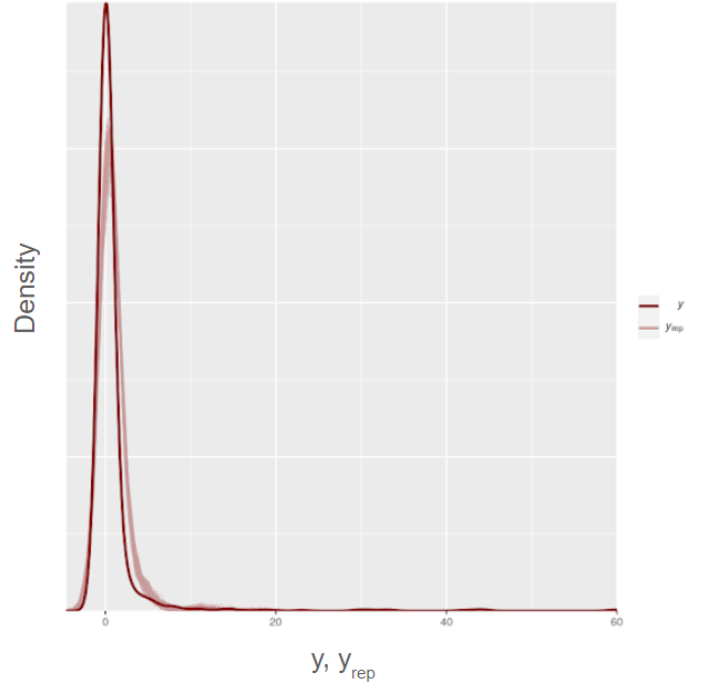
The distribution of the DV looks as follows:
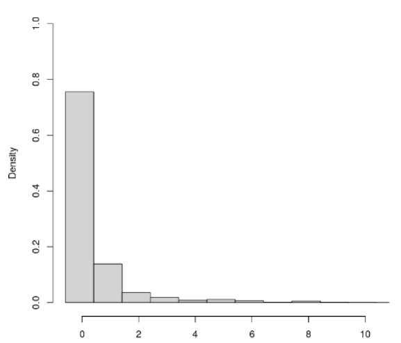
This is a variance decomposition analysis. The effects of interest are the variance components of the three nested hierarchical levels.
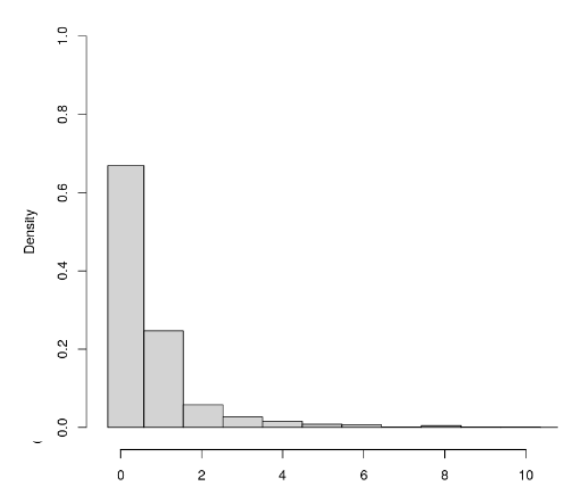
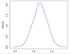
The control control variable has a similar right skewed shape.
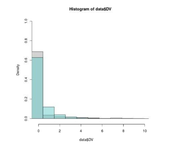
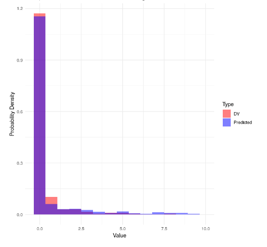
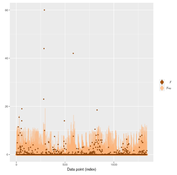
The predicted posterior (turkoise in the figure below) seems to fit reasonably well with the actual distribution of the DV(gray in the below figure) (the histogram is cut off on the right to zoom in more here).
The results of our conventional (linear hierarchical) model are as follows (the alternative models have similar results):
- Variance explained level 1: 2.9
- Variance explained level 2: 5.1
- Variance explained level 3: 5.3
- Variance explained control variable: 0.9
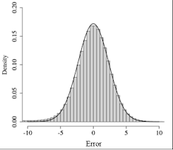
The distribution of the error term (posterior of DV - DV) looks as follows:
R heat for all variables is between 1.000 and 1.003 Effective samples size is > 1000 for every variable.
The normal model seems to converge well after some initial period (warm up is 2000 and sampling is 2000). Below, two markov chains after the warm up are shown (we ran 4 chains but the image is difficult to read with 4 chains).
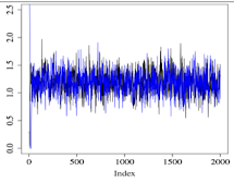
Another view of the distribution of two markov chains:
We also ran the model with t-distributed priors for the random effects, with t-distributed errors and with random effects that can vary for each level of the hierarchy and obtained similar results.
The estimates for the variance components that we obtain stay roughly the same.
Finally running a model with a Tweedie link function gives similar results for the variance components (see my other post here).
The details of the Tweedie model we ran can be found here. Note that the Tweedie model linked in here allows the random effects for each level to be drawn from different standard deviations. The convergence of the Tweedie model and its posterior also look good and we can provide them if this is helpful.
Finally, we noticed that the confidence intervals of the variance estimates of all models seem to be much wider than the confidence intervals of point estimates and asked in a post in this forum, whether this is normal and to be expected.
The posterior predicted DV vs actual DV for the Tweedie model looks as follows.
Great, now there was enough details. All look good. You could get even better comparison of model predictions and actual data by using square root transformation for the x-axis, or by using PIT-ECDF plots (see PPC distributions — PPC-distributions • bayesplot). Also with that many “random effects”, it would be useful to check LOO-predictive checks, too. See Roaches cross-validation case study, especially Section 4 which illustrates how a model with many vying intercepts (“random effects”) can look too good in posterior predictive checks.
Thank you very much for your suggestion.
Results for the “standard” normal hierarchical model
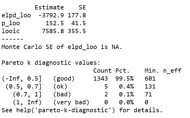
LOO diagnostic results
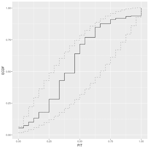
PIT-ECDF plot of the normal model (99% confidence interval)
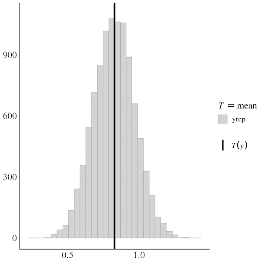
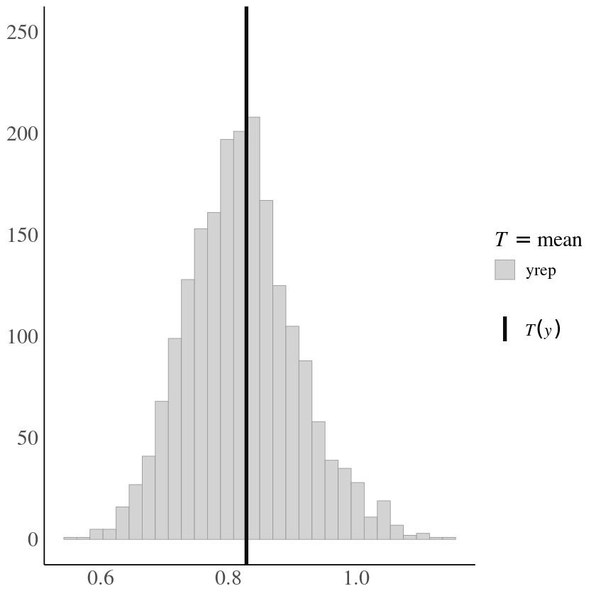
Mean of the data vs generated means
.
The approximate leave-one-out (LOO) cross-validation for the normal model using Pareto smoothed importance sampling (PSIS) gives a p_loo = 152.5, which is smaller than p = 276, the total number of parameters of the model. p_loo = 152.5 is also smaller than the total number of observations N/5 (1350/5 =270). For 99.5% of samples (n=1343) k<0.5. There are 5 samples (0.4%), where 0.5<k<0.7 and 2 samples (0.1%) where 0.5<k<1. There is no sample where k >1.
The PIT-ECDF shows that the distribution of the data lies within the 99% confidence interval of the distribution generated by the model. The normal model also generates means of the data that fit with the overall mean of the distribution
Results for the Tweedie hierarchical model
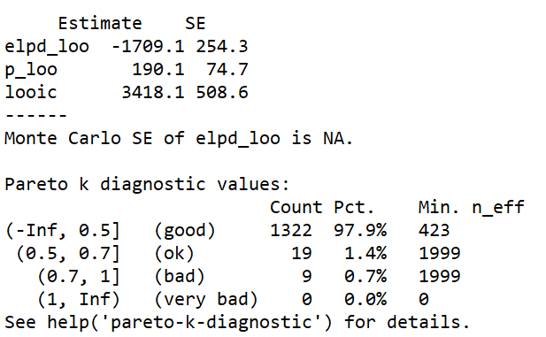
LOO diagnostic results
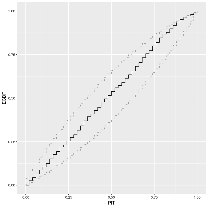
PIT-ECDF plot of the normal model (99% confidence interval)
Mean of the data vs generated means
The approximate leave-one-out (LOO) cross-validation for the Tweedie model using Pareto smoothed importance sampling (PSIS) gives a p_loo = 190.1 which is smaller than p = 276, the total number of parameters of the model. p_loo = 190.1 is also smaller than the total number of observations N/5 (1350/5 =270). For 97.9% of samples (n=1322) k<0.5. There are 19 samples (1.4%), where 0.5<k<0.7 and 9 samples (0.7%) where 0.5<k<1. There is no sample where k >1.
The PIT-ECDF shows that the distribution of the data lies within the 99% confidence interval of the distribution generated by the Tweedie model. The Tweedie model also generates means of the data that fit with the overall mean of the distribution.
Comparison of the models:
- Both, the normal hierarchical random effects model and the Tweedie hierarchical random effects model seem to fit with the data, and, given the above diagnostics, it may not be surprising that they generate similar results for the variance decomposition analysis
- Whilst the Tweedie model performs better on the PIT-ECDF plot, according to the pareto k diagnostic values, the normal model is less sensitive to particular values of the data
- The p_loo of the Tweedie model (p_loo = 190.1) implies that it has a higher risk of overfitting than the normal model (p_loo = 152.5), which can be expected, given that the Tweedie model is more flexible.
- The looic of the Tweedie model (3418.1) which is less than half of the looic of the normal model (7585.8) implies that, nevertheless, overall the Tweedie model seems to be a better fit with the data
Thank you for the feedback. This was really helpful. The Interaction on the forum gave us confidence that the set-up and interpretation of the results are valid, especially as the effect magnitudes are similar across both models. We have been thinking how to present the results to an audience outside of the field of statistics. To us it seems that because the results of both models are similar, it might be better to present the simpler model as our main results and the Tweedie as a robustness check. Do you think this is a reasonable approach?
Great, this is nice report
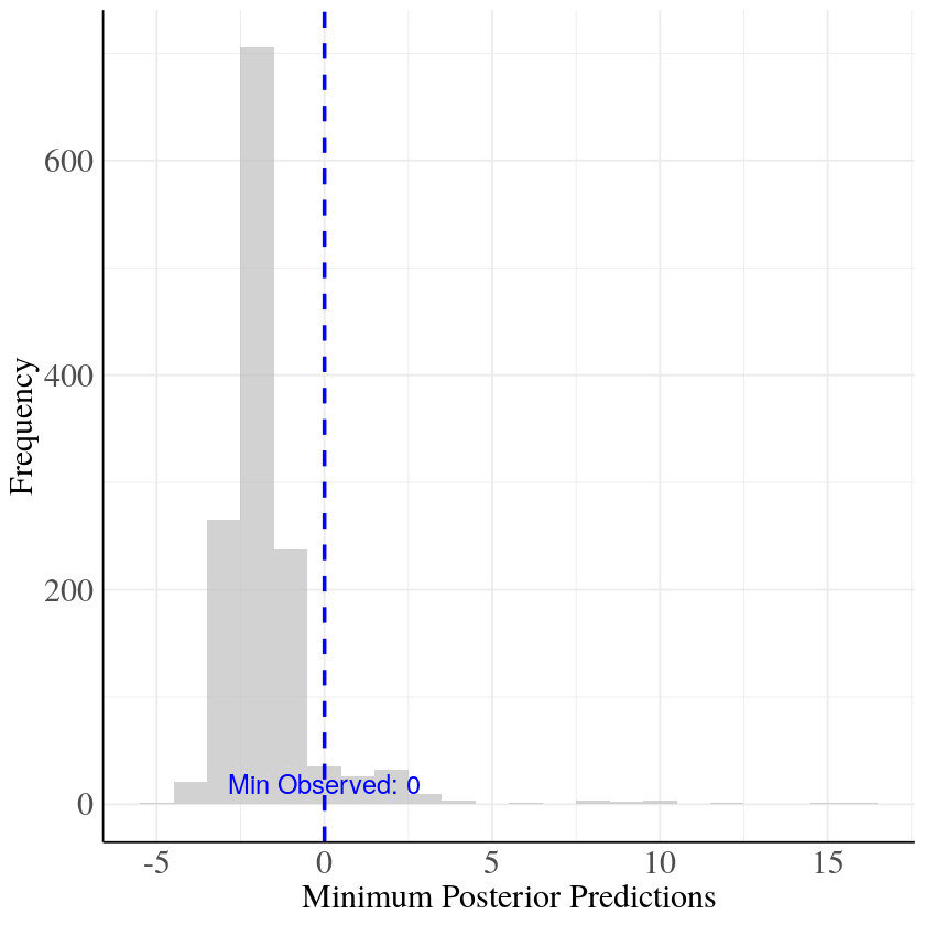
This is usually very weak diagnostic, as the model can learn the mean easily. Min and max test statistics would be better.
As they both stay within the envelope, there is no difference. Why the plot for normal has fewer steps?
You could also check ppc_dens_overlay, ppc_loo_intervals, and ppc_loo_pit_qq (we’ll add ppc_loo_pit_ecdf soon)
The difference in elpd_loo is so big, that I would be interested in seeing those other plots, too, to better understand where the difference in predictive performance might come from.
Thank you so much for your comment. The additional analysis for the “normal” model and the “Tweedie” model with which we identify the explained variance at each level are below.
Additional posterior analyses for our two variance decomposition models:
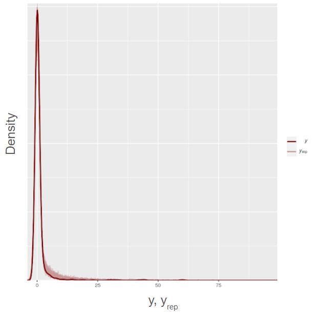
Dense overlay normal
Dense overlay Tweedie
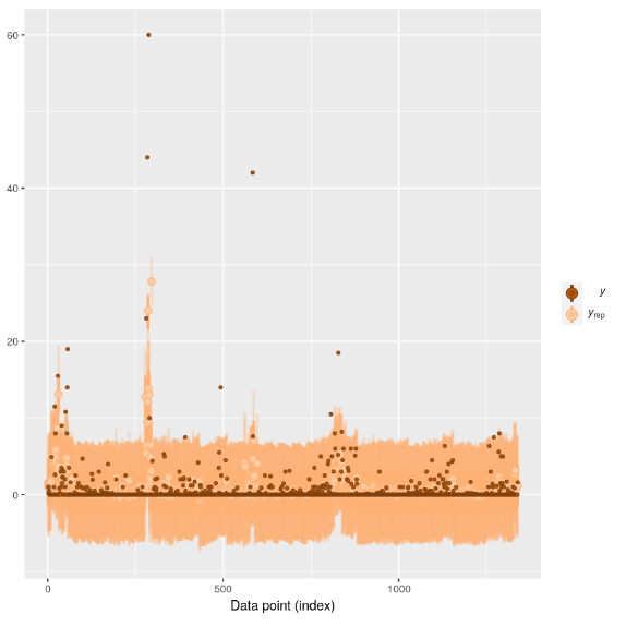
ppc_loo_interval_Normal
ppc_loo_interval_Tweedie
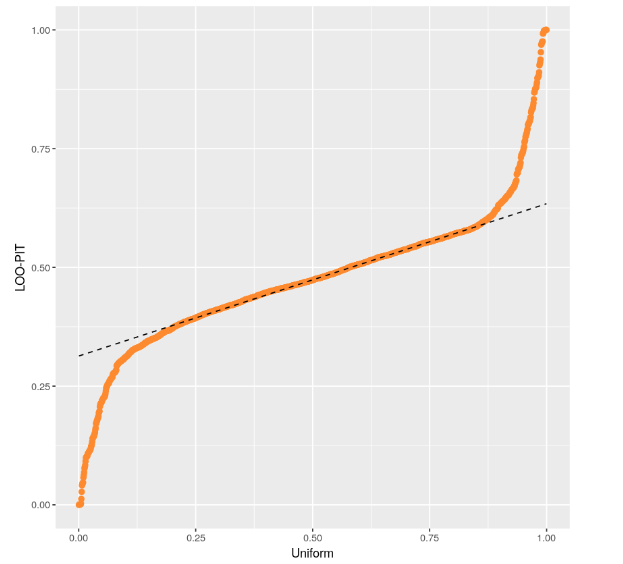
Normal_ppc_loo_pit
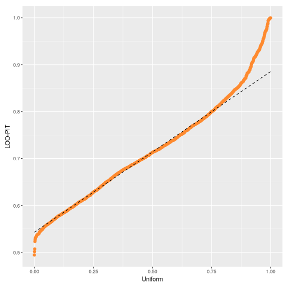
Tweedie_ppc_loo_pit
Extreme Value statistics:
Min observed value Normal distribution
Max value normal distribution
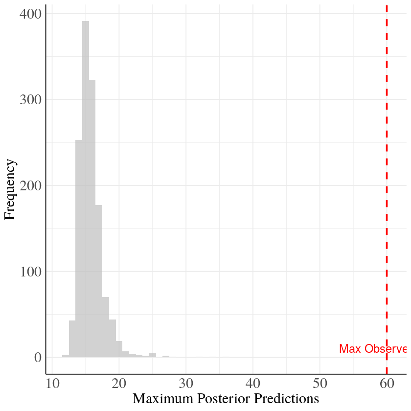
We ran robustness checks winsorizing the data including a cut-off value of 20. The winsorized models produce the same variance components as the original model.
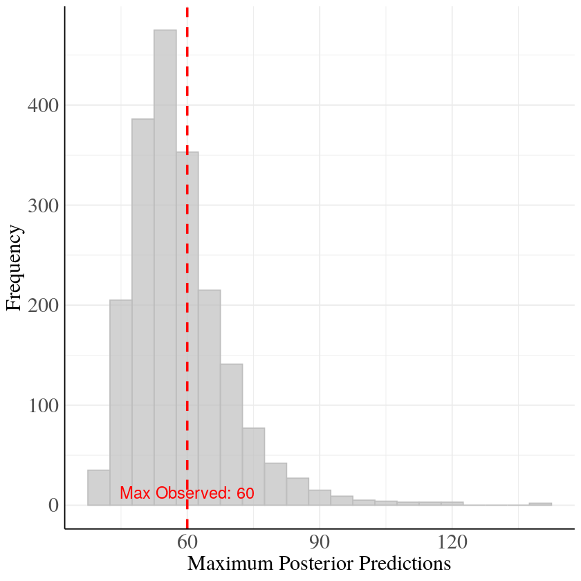
For the Tweedie distribution, by definition, the minimum value is always zero, so below we show a distribution of zeros for different draws of the model compared to the number of zero observations in the dependent variable.
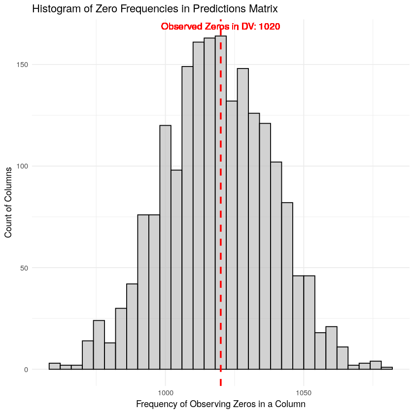
Max Value Tweedie distribution
Cool Tweedie model is clearly better. You can improve density overlay plots by adding the following after the plot function call
+ scale_x_sqrt()
and for the interval plots add
+ scale_y_sqrt()
These will apply square root transformation for axes, so that it is easier to see details both near 0 and in the tail.
It seems you are using an old version of bayesplot. You would get better ppc_loo_pit plots with the latest CRAN release, or at least add the following to get the correct diagonal line.
+ geom_abline()
Although the Tweedie model is better the LOO-PIT plot shows it’s not perfect. I did guess correctly that the Posterior PIT-ECDF was too good due to double use of data and flexible model. LOO-PIT plot shows that the Tweedie model is slightly overdispersed compared to the data.
Thank you so much for your insightful comments. I will adjust the visualization of the
charts according to your suggestions. To recap, the Tweedie model performs well in
terms of the convergence checks, mean of the distribution, zero inflation, dense
overlay, PIT-ECDF and when we plug in the estimated phi, mu and theta it recovers
the real variance of the DV. As you point out, on the ppc_loo_pit, the Tweedie shows a
slight overdispersion.
I wonder to which extent the overdispersion of the Tweedie model influences
our analysis given the purpose of our study: Our DV is start-up funding. It is right
skewed - most start-ups secure little or no funding, but a few get substantial amounts.
For the purpose of our investigation, we are less concerned whether the model
estimates extreme amounts of funding precisely. The sheer fact that a start-up
secured a high amount of funding is considered a success.
It sounds like it is only you who can assess which imperfections don’t matter for you? Are you using this for making decisions, or are you just reporting historical behavior?
Thank you very much @avehtari. We are reporting historical behaviour.
In that case there is not bug danger in making bad decisions, and you can report the deficiencies of the model (that is, it’s not predicting the tails well)
Hi avehtari.
Given that the Tweedie model was slightly over dispersed we thought that an additional analysis following your 2021 paper about probabilistic outlier identification might help. We followed that approach and were curious whether we should present it along the other tests you suggested.
Following the approach results stay similar to the previous ones and our LOO PIT Plot now looks like this:

I think it makes sense since if you provide the result without and with it, it will provide more information about the model behavior. It is fine to acknowledge that the model is not perfect and is not modeling the extreme cases well.