Consultation regarding max_treedepth, and poor mixing of some chains in a hierarchical computational learning mode

Dear all.

I’m trying to fit a quite complex semi-Bayesian human learning computational model to participant’s data (or simulated data).
The model itself is quite complex, and I use a user-defined function to code it, and this part works quite well. The simplest model has two free parameters - GD and LD. These parameters are generally limited from -1 to 1. When coding a simple STAN model for a single participant, I use Phi_approx with an additional transformation to reach these bounds, and it usually works quite well (good mixing). This the model I used for single participants that works:

    parameters{
         real GD0;
         real LD0;
    }

    transformed parameters{
         real GD;
         real LD;
         GD=2*(Phi_approx(GD0)-0.5); 
         LD=2*(Phi_approx(LD0)-0.5);
         // the 2 and -0.5 are used to create parameters bounded from -1 to 1 instead of 0 to 1
    }

    model{
        vector [nTrials] pRight1;
        lamdaDepletion0~normal(0,0.3);
        gammaDepletion0~normal(0,0.3);
        // I used SD of 0.3 instead of 1 because I want to create a distribution with more mass on values around 
        zero, and low mass on values close to 1 and -1.

        pRight1=Bmodel(dataValues,GD,LD);
        //Bmodel is the model itself, and the other values are just data. It produces a single value - the probability of a right arrow response by a participant, which is then used for the bernoulli likelihood below. 

        Response~bernoulli(pRight1);

    }

So this model works pretty well. However, when I try to implement a hierarchical model for all participants using non-central parameterization as follows I always get warnings regarding max_treedepth exceeded, and poor mixing (see below). This is how I am trying to implement the hierarchical model:

    parameters{
        real GD0[nSubj];
        real LD0[nSubj];
        real GD0_MU;
        real LD0_MU;
        real <lower=0> GD0_SD;
        real <lower=0> LD0_SD;
    }

    transformed parameters{
         vector [nSubj] GD;
         vector [nSubj] LD;
         GD=2*(Phi_approx(GD0_SD*to_vector(GD0)+GD0_MU)-0.5);
         LD=2*(Phi_approx(LD0_SD*to_vector(LD0)+LD0_MU)-0.5);
    }


    model{
         vector [nTrials] pRight1[nSubj];
         LD0_MU~normal(0,0.3);
         GD0_MU~normal(0,0.3);
         LD0_SD~normal(0,0.1)T[0,];
         GD0_SD~normal(0,0.1)T[0,];

         LD0~normal(0,1);
         GD0~normal(0,1);

         for (s in 1:nSubj){
           pRight1[s]=Bmodel(dataValues,GD[s],LD[s]);
           Response[s]~bernoulli(pRight1[s]);
         }
    }

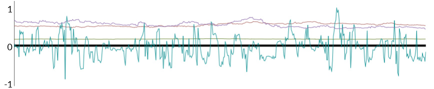
Here is an example of a typical result for the latter model (Clearly only Chain 3 works. The others just stay stuck, and do not mix). I’ve tried decreasing adapt_delta to 0.6, and increase max_treedepth - but that didn’t do the job. I even tried adding jitter to the step size - still did not work.
I appologize for not inserting the full model but it is very long, and I don’t think anyone would like to get into it just to answer my question. Nonetheless any help would be appreciated.


Thanks,
Isaac

With lots of data, the centered parameterization works better as the non-centered one turns into a comma-shaped funnel. We’re going to write this all up in general, but I’d suggest just trying to fix that.

Second, try initializing with smaller step sizes and increasing adapt delta. That’ll make adaptation try a lot harder to not diverge.

You can improve the model efficiency by dropping the truncation here:

LD0_SD~normal(0,0.1)T[0,];

it’s not needed given that the arguments to normal (0 and 0.1) are constant.

If you don’t care about the shape of Phi_approx, it’s just a rescaled inv_logit. The efficient built-in to convert (-infinity, infinity) to (-1, 1) is tanh.

You can also declare and define in one line, e.g.,

vector [nSubj] GD = tanh(GD0_SD * GD0 + GD0_MU);

and drop the to_vector by just declaring GD0 as a vector initially.

Dear Bob.

Thank you for all the advice. The efficiency advice worked well, however, unfortunately, the advice regarding the mixing problems (increasing adapt delta and decreasing stepsize) seems to make things worse, as now all chains were stuck at one value, with no mixing at all. I can say that when running the model on single participants, using lower adapt delta (0.6 and even lower) worked better. How would you interpret such a situation? Is there anything to do about it?

Thanks again!

Isaac.

With lower adapt_delta, the adapted step size will be larger. This will make it less likely to get stuck, but more likely to diverge. Were you getting divergences with adapt_delta = 0.6?

The likely situation is that with larger step sizes, you’re failing to find the problematic portions of the posterior and hence generating biased answers. You can uncover this with simulation-based calibration, even done informally.

Most samplers, like Gibbs or Metropolis or ensemble methods, will fail to find the problematic part of the posterior, such as the neck of the funnel in a centered hierarchical parameterization.

People often erroneously conclude that NUTS is broken, but what’s really happening is that NUTS is discovering the pathologies that other samplers miss. Unfortunately, NUTS can’t always sample once discovering the pathologies. Riemannian HMC can handle a lot of these cases, but it’s very expensive and we don’t have a well-tested implementation of higher-order derivatives yet.

So my guess is that there’s some highly varying curvature in your model (the Hessian matrix varies at different locations in the posterior, as with funnel or banana shapes) that needs to be reparameterized in order to be fit. You may be able to see that by plotting the output of warmup or sampling with larger step sizes, where basic funnel and banana shapes will become apparent (we sample on the unconstrained scale, so you need to transform back to see these).