If I calculate exact LOO CV for flagged observations with too high Pareto k diagnostics (e.g. >0.7) and calculate the exact elpd as exact_elpd=log(mean(exp(llExactLoo))), where llExactLoo contains the sampled predictive likelihood of the left out observation, can I still use the compare function? If my PSIS-LOO CV estimates are denoted LOO1 and i is the observation flagged as problematic, is it sufficient to replace the value in LOO1$pointwise[i,1] with exact_elpd and run compare(LOO1,LOO2), where LOO2 is the equivalent LOO object for a different model (which may or may not also include exact eldp for some observation(s))?
1 Like
If llExactLoo is computed correctly (if you post the Stan code, I can check that), then
yes. In more recent loo versions, it’s loo_compare
That is what loo does for rstanarm and brms models when using k_threshold or refit options.
Yes, but use loo_compare
Thanks avehtari, and that’s a very kind offer to check the stan code! It’s somewhat messy because it has a bunch of optional parameters that can be included or excluded (thus the need for loo cv model selection). The parts used for loo are under generated quantities, where log_lik either is the likelihood of all N observations (when doexactloo is FALSE) or the left out observation (when doexactloo is TRUE). I tried the exact elpd also for non-flagged observations, and the estimates are consistently very close to the PSIS-LOO CV elpd.
Also, since there are too many potential model combinations to compare, my plan was to
- Run the full model
- Run models where one factor at the time is excluded
- Use LOO CV to identify which factors increase elpd when they are removed
- Run the model with all factors identified in step 3 removed to ensure that elpd is improved compared to the full model when all identified factors are removed.
Does that seem like a reasonable approach to you?
data {
  int<lower=1> N;
  real<lower=0> logAge[N];
  real<lower=0> Diam[N];
  real<lower=0> Height[N];
  real<lower=0> Bonitet[N];
  real<lower=0> SoilDepth[N];
  real<lower=0> Prunes[N];
  int<lower=1> SoilType[N];
  int<lower=1> NSoilTypes;

  int<lower=0, upper=1> includeDiam;
  int<lower=0, upper=1> includeHeight;
  int<lower=0, upper=1> includeBonitet;
  int<lower=0, upper=1> includeSoilDepth;
  int<lower=0, upper=1> includePrunes;

  int<lower=0, upper=1> includeSoilType;

  int<lower=0, upper=1> includeDiamExp;
  int<lower=0, upper=1> includeHeightExp;
  int<lower=0, upper=1> includeBonitetExp;
  int<lower=0, upper=1> includeSoilDepthExp;
  int<lower=0, upper=1> includePrunesExp;


  real<lower=0> SIGMADiam;
  real<lower=0> SIGMAHeight;
  real<lower=0> SIGMABonitet;
  real<lower=0> SIGMASoilDepth;
  real<lower=0> SIGMAPrunes;

  real<lower=0> SIGMAlogsigma0;
  real<lower=0> SIGMAsigmacoef;

  real<lower=0> DiamAlpha;
  real<lower=0> HeightAlpha;
  real<lower=0> BonitetAlpha;
  real<lower=0> SoilDepthAlpha;
  real<lower=0> PrunesAlpha;

  int<lower=0, upper=1> doexactloo;
  real logAgePred[doexactloo ? 1 : 0];
  real DiamPred[doexactloo ? 1 : 0];
  real HeightPred[doexactloo ? 1 : 0];
  real BonitetPred[doexactloo ? 1 : 0];
  real SoilDepthPred[doexactloo ? 1 : 0];
  real PrunesPred[doexactloo ? 1 : 0];
  int<lower=1> SoilTypePred[doexactloo ? 1 : 0];

}


parameters {
  real DiamCoef[includeDiam ? 1 : 0];
  real HeightCoef[includeHeight ? 1 : 0];
  real BonitetCoef[includeBonitet ? 1 : 0];
  real SoilDepthCoef[includeSoilDepth ? 1 : 0];
  real PrunesCoef[includePrunes ? 1 : 0];
  real SoilTypeCoef_raw[includeSoilType ? NSoilTypes : 0];

  real<lower=0> DiamExp[includeDiamExp ? 1 : 0];
  real<lower=0> HeightExp[includeHeightExp ? 1 : 0];
  real<lower=0> BonitetExp[includeBonitetExp ? 1 : 0];
  real<lower=0> SoilDepthExp[includeSoilDepthExp ? 1 : 0];
  real<lower=0> PrunesExp[includePrunesExp ? 1 : 0];

  real logsigma0;
  real sigmacoef;

  real intercept;
  real<lower=0> SIGMASoilType[includeSoilType ? 1 : 0];
}

transformed parameters {
  real mu[N];
  real<lower=0> sigma[N];
  real SoilTypeCoef[includeSoilType ? NSoilTypes : 0];
  real DiamContrib[N];
  real HeightContrib[N];
  real BonitetContrib[N];
  real SoilDepthContrib[N];
  real PrunesContrib[N];
  real SoilTypeContrib[N];
  real mupred[doexactloo ? 1 : 0];
  real sigmapred[doexactloo ? 1 : 0];
  real DiamContribPred[doexactloo ? 1 : 0];
  real HeightContribPred[doexactloo ? 1 : 0];
  real BonitetContribPred[doexactloo ? 1 : 0];
  real SoilDepthContribPred[doexactloo ? 1 : 0];
  real PrunesContribPred[doexactloo ? 1 : 0];
  real SoilTypeContribPred[doexactloo ? 1 : 0];

  if (includeDiam){


    for (i in 1:N){
      if (includeDiamExp){
        DiamContrib[i]=DiamCoef[1]*Diam[i]^DiamExp[1];
        if (doexactloo){

          DiamContribPred[1] = DiamCoef[1]*DiamPred[1]^DiamExp[1];
        }

      }else{

        DiamContrib[i]=DiamCoef[1]*Diam[i];
        if (doexactloo){

          DiamContribPred[1] = DiamCoef[1]*DiamPred[1];
        }
      }

    }

  }else{
    for (i in 1:N){

      DiamContrib[i]=0;
      if (doexactloo){

        DiamContribPred[1] = 0;
      }
    }

  }

  if (includeHeight){


    for (i in 1:N){
      if (includeHeightExp){
        HeightContrib[i]=HeightCoef[1]*Height[i]^HeightExp[1];
        if (doexactloo){

          HeightContribPred[1] = HeightCoef[1]*HeightPred[1]^HeightExp[1];
        }

      }else{

        HeightContrib[i]=HeightCoef[1]*Height[i];
        if (doexactloo){

          HeightContribPred[1] = HeightCoef[1]*HeightPred[1];
        }
      }

    }

  }else{
    for (i in 1:N){

      HeightContrib[i]=0;
      if (doexactloo){

        HeightContribPred[1] = 0;
      }
    }

  }

  if (includeBonitet){


    for (i in 1:N){
      if (includeBonitetExp){
        BonitetContrib[i]=BonitetCoef[1]*Bonitet[i]^BonitetExp[1];
        if (doexactloo){

          BonitetContribPred[1] = BonitetCoef[1]*BonitetPred[1]^BonitetExp[1];
        }

      }else{

        BonitetContrib[i]=BonitetCoef[1]*Bonitet[i];
        if (doexactloo){

          BonitetContribPred[1] = BonitetCoef[1]*BonitetPred[1];
        }
      }

    }

  }else{
    for (i in 1:N){

      BonitetContrib[i]=0;
      if (doexactloo){

        BonitetContribPred[1] = 0;
      }
    }

  }

  if (includeSoilDepth){


    for (i in 1:N){
      if (includeSoilDepthExp){
        SoilDepthContrib[i]=SoilDepthCoef[1]*SoilDepth[i]^SoilDepthExp[1];
        if (doexactloo){

          SoilDepthContribPred[1] = SoilDepthCoef[1]*SoilDepthPred[1]^SoilDepthExp[1];
        }

      }else{

        SoilDepthContrib[i]=SoilDepthCoef[1]*SoilDepth[i];
        if (doexactloo){

          SoilDepthContribPred[1] = SoilDepthCoef[1]*SoilDepthPred[1];
        }
      }

    }

  }else{
    for (i in 1:N){

      SoilDepthContrib[i]=0;
      if (doexactloo){

        SoilDepthContribPred[1] = 0;
      }
    }

  }

  if (includePrunes){


    for (i in 1:N){
      if (includePrunesExp){
        PrunesContrib[i]=PrunesCoef[1]*Prunes[i]^PrunesExp[1];
        if (doexactloo){

          PrunesContribPred[1] = PrunesCoef[1]*PrunesPred[1]^PrunesExp[1];
        }

      }else{

        PrunesContrib[i]=PrunesCoef[1]*Prunes[i];
        if (doexactloo){

          PrunesContribPred[1] = PrunesCoef[1]*PrunesPred[1];
        }
      }

    }

  }else{
    for (i in 1:N){

      PrunesContrib[i]=0;
      if (doexactloo){

          PrunesContribPred[1] = 0;
        }
    }

  }

  if (includeSoilType){

    for (t in 1: NSoilTypes){
      SoilTypeCoef[t]=SoilTypeCoef_raw[t] * SIGMASoilType[1];// reparametrisation of chi for improved computation

    }

    for (i in 1:N){


      SoilTypeContrib[i]= SoilTypeCoef[SoilType[i]];
      if (doexactloo){

          SoilTypeContribPred[1] = SoilTypeCoef[SoilTypePred[1]];
        }

    }
  }else{
    for (i in 1:N){

      SoilTypeContrib [i]= 0;

      if (doexactloo){

          SoilTypeContribPred[1] = 0;
        }

    }

  }

  for (i in 1:N){
    mu[i]=intercept + DiamContrib[i] + HeightContrib[i] + BonitetContrib[i] + SoilDepthContrib[i] + PrunesContrib[i] + SoilTypeContrib[i];
    sigma[i]=exp(logsigma0+sigmacoef*mu[i]);
  }

  if (doexactloo){
    mupred[1] =intercept + DiamContribPred[1] + HeightContribPred[1] + BonitetContribPred[1] + SoilDepthContribPred[1] + PrunesContribPred[1] + SoilTypeContribPred[1];
    sigmapred[1]=exp(logsigma0+sigmacoef*mupred[1]);

  }

}
model {
  for (i in 1:N){

    logAge[i] ~ normal(mu[i], sigma[i]);

  }

  if (includeDiam){

    DiamCoef[1] ~ normal(0,SIGMADiam);
    if (includeDiamExp){

      DiamExp[1] ~ lognormal(0,DiamAlpha);


    }

  }

  if (includeHeight){

    HeightCoef[1] ~ normal(0,SIGMAHeight);

    if (includeHeightExp){

      HeightExp[1] ~ lognormal(0,DiamAlpha);


    }
  }

  if (includeBonitet){

    BonitetCoef[1] ~ normal(0,SIGMABonitet);
    if (includeBonitetExp){

      BonitetExp[1] ~ lognormal(0,DiamAlpha);


    }

  }

  if (includeSoilDepth){

    SoilDepthCoef[1] ~ normal(0,SIGMASoilDepth);

    if (includeSoilDepthExp){

      SoilDepthExp[1] ~ lognormal(0,DiamAlpha);


    }
  }

  if (includePrunes){

    PrunesCoef[1] ~ normal(0,SIGMAPrunes);

    if (includePrunesExp){

      PrunesExp[1] ~ lognormal(0,DiamAlpha);


    }
  }

  if (includeSoilType){
    for (t in 1:NSoilTypes){
      SoilTypeCoef_raw[t] ~ normal( 0 , 1 ); //  reparametrisation for improved computation
      //SoilTypeCoef[t] ~ normal(0,SIGMASoilType[1]);

    }

    SIGMASoilType[1] ~ cauchy(0,1);


  }


  logsigma0 ~ normal(0,SIGMAlogsigma0);
  sigmacoef ~ normal(0,SIGMAsigmacoef);
}

generated quantities {
  vector[doexactloo ? 1 : N] log_lik;
  if (doexactloo){
    log_lik[1] = normal_lpdf(logAgePred[1]|mupred[1] , sigmapred[1]);

  }else{
    for (i in 1:N){

      log_lik[i] = normal_lpdf(logAge[i]|mu[i] , sigma[i]);

    }


  }


}No problem, it’s often the fastest way to be certain :)
I assume you then when you call stan with doexactloo, you will pass data with the one observation removed from logAge etc and that one observation is passed as logAgePred etc.
With quite small amount of models to compare, this is safe.
It is unlikely that elpd would increase if you remove something.
If you have reasonable priors or N is bigger than the total number of parameters and
- you remove a factor with no useful predictive information, elpd stays about the same
- you remove a factor with some useful predictive information, elpd gets lower unless the removed factor is correlated with some of the remaining factors
You could make the model code simpler by passing the data as a matrix, define Coefs and Exps as vectors, have transformed matrix with certain columns exponentiated with Exps and then get mu as vector times matrix.
I’m curious about the model. What is the justification for Exps? Is sigma strongly dependent on mu even your have taken logarithm of Age? How do PPC plots look like?
Yes, indeed I pass the data without the left-out observation, meaning N will be 1 lower than when I call stan with doexactloo=FALSE.
Hmm… My impression was that the inclusion of factors without predictive information would add additional uncertainty that would reduce elpd of left-out observations (either exact or PSIS-LOO), thus punishing the model for being over-parameterized. If the removal of redundant factors doesn’t increase elpd, then wouldn’t the best predictive model always be the one that includes everything? You’ve left me confused. Thank you :)
[/quote]
The model is attempting to predict the age of trees based on observations that doesn’t require drilling into the core. The logarithm of age doesn’t necessarily grow linearly with the explaining factors, and rather than making assumptions about what transformation might be appropriate, I wanted to see if I could estimate the powers that gave the best fit. The way it turns out, however, is that only diameter has an obvious; if I look at 95% credibility intervals of all other coefficients, all of them envelope 0. So attempting to estimate the exponents for the other ones is a lost cause. So I might skip the exponents and just log-transform the diameter data, but it would be interesting to see if the power transformation with estimated exponents does better than an a priori specified transformation.
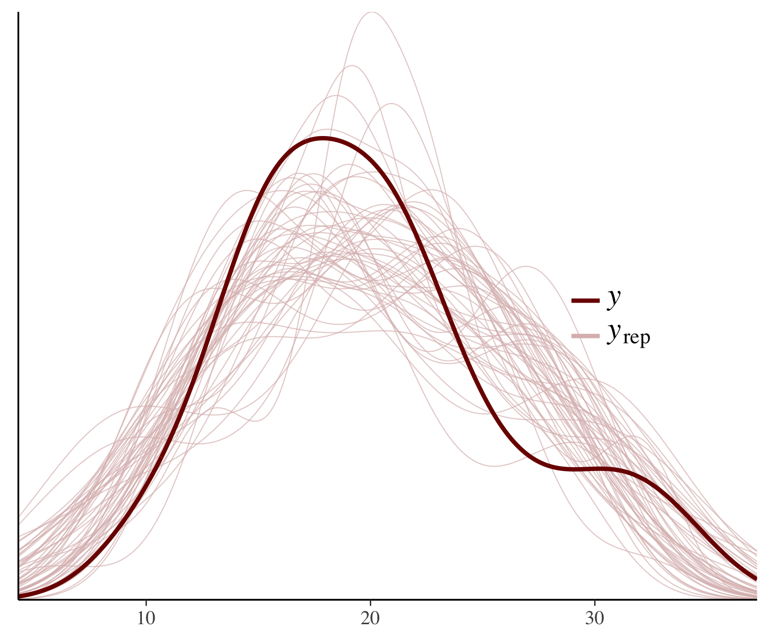
Not sure what PPC plot is appropriate, but here are some violin plots based on a model excluding everything but diameter. I’ve predicted logAge based on the predictive data for each tree and grouped them by diameter classes (<30cm, 30-50 cm, >50cm). The distribution of both predictive distributions and data is wider in the narrowest class (a). It also makes some biological sense. Only old trees can be wide, but trees can grow slow for various reasons, so narrow trees can be both young and old.
Your input is highly appreciated!
That is the old folklore for maximum likelihood. This is much less likely to happen if we can integrate over the posterior accurately. If the integration works, I’ve seen only extreme examples where this would happen and some of them have silly priors. I have seen this also if the integration approximation fails. See also Comparison of Bayesian predictive methods for model selection | Statistics and Computing and Model selection tutorials and talks
Usually it is the best, and if not you should think harder about your priors and prior predictive simulation. See, e.g. Sparsity information and regularization in the horseshoe and other shrinkage priors, [1810.02406] Projective Inference in High-dimensional Problems: Prediction and Feature Selection, and Visualization in Bayesian Workflow | Journal of the Royal Statistical Society Series A: Statistics in Society | Oxford Academic.
I recommend to use splines or GPs for unknown non-linearities. It’s easy with rstanarm and brms. Exp would make sense only if there would be physical model with such parameter.
Did you forgot to upload them?
Have you looked at plots that bayesplot provides?
I’ve read these papers. Will do it again. It bothers me that “include everything” would always be the best option; then I might as well include the zodiac sign of the landowners where each data point was collected. But I guess the strictly Bayesian view is that I (should) have some reasonable prior belief about how much such a factor would explain that I could incorporate in the analysis.
If you don’t mind me asking, why do you think exponents make no sense. My only worry is that the units become problematic and it’s difficult to elicit reasonable priors for the associated coefficients. But for predictive purposes, it seems pretty reasonable to me–it ends up with a monotonically increasing/decreasing transformation with linear (no transformation) as a special case.
oops. These are made with Bayesplot.

That also applies in the current case where the exponent of the transformation is estimated as well, except now you’re averaging over a bunch of different scalings.
But that sorta happens with any non-linear transformation. You’re in a situation where you have:
y = A * f(x)
And so it’s just not gonna be feasible to think about A in terms of the units of y and x.
That doesn’t mean it’s impossible to get reasonable priors. You can choose your priors based on the scales of y and f(x).
But I don’t think you’d even have a separate A like that in brms. It’s probably built in somewhere. It is with GPs.
I hope that wasn’t too wishy-washy to be useless.
Cool. And good to know they don’t make this point clear enough.
Include everything 1) you assume might have non-negligible predictive relevance and 2) use reasonable distributions to describe the uncertainty of their relevance.
- If you are uncertain then Bayes theory says that you need to integrate over all your uncertainties. If you are certain that zodiac sign doesn’t have predictive relevance it’s ok to leave that out. If you are certain that some factor have physically justified causal effect, but that effect is negligible it’s ok to leave that out.
- With just few factors and lot of data, the results are not that sensitive to priors. More you add more you need to think. When adding more and more things that might have relevance you need to choose the prior so that the prior predictive distribution stays in a reasonable range, which means that you can’t have vague independent priors for all the new factors you are adding (Piranha problem theorem says that you can’t have a large number of independent effects). Either you should use prior (like (regularized) horseshoe with our hyperprior recommendations) which says that only small number of factors are relevant, but you don’t know which, or you should use prior that say many factors are relevant but correlating (like SPC model we used in other paper), or you should have prior on signal noise ratio (e.g. prior on R^2 as in
stan_lm). Given such priors it’s less likely that adding more covariates makes predictions worse, and even if oracle would tell you how many factors are relevant but you don’t know which, it’s better to include more factors and integrate over the uncertainty.
Of course it is possible to make counter examples, but when you start looking at the assumptions made they have to be silly to have strong undesired behavior.
I like that you ask if something I say is not clear. Because you didn’t give physical explanation for them and you were uncertain about the functional shape. In such case you should not choose any specific functional shape, but use flexible non-parametric models.
Selecting reasonable prior for scale parameters for additive non-linear components is similar to selecting priors for linear models. I’m worried that exp doesn’t have meaning and that there is identifiability issue so that you should define joint prior for the coefficient and exponent term, but I don’t know good solutions for that.
You can have that with splines and GPs, too. Linear as special case is in gamms in brms and rstanarm, if monotonicity constraint is needed it requires little extra work, but I would try first without it.
How about something like this https://mc-stan.org/assets/img/bayesplot/ppc_dens_overlay-rstanarm.png ?
1 Like
Didn’t know about this paper until now. Just skimmed it. Cool stuff!
So instead of doing a regression on X you do a regression on Z = XW which is nice computationally because you have way fewer variables in your regression and you can always transform the coefficients back via \beta = W \tilde{\beta}. I have a question though. In the paper you guys used a horseshoe prior. Was the horseshoe prior on the transformed coefficients, i.e. \tilde{\beta} \sim N(0, \tau^2 \Lambda),
or on the original coefficients i.e. \beta = W \tilde{\beta} \sim N(0, \tau^2 \Lambda)?
Ideally, you’d want sparsity on the original untransformed \beta scale, and you can surely write a model in Stan with the second statement, but I’m not sure if the second statement is legitimate.
I was referring to this paper [1810.02406] Projective Inference in High-dimensional Problems: Prediction and Feature Selection
where “we use nc = 3 SPCs with a Gaussian prior N”
It seems you read this older paper Iterative Supervised Principal Components
where we use regularised horseshoe prior.
Only if we assume that only small number of features are relevant, but we are using SPCA when we assume that there can be groups of correlating features. In the earlier paper we selected the number of components automatically which could lead to quite many components in some tested methods and then RHS prior could be useful. In the later paper we used so few components that RHS is not better than N. In both papers the focus for the models using SPCA was just good prediction, and in the latter the feature relevance is decided using decision theoretical predictive projection approach.
2 Likes