So I am trying to fit a relatively simple GLMM with a single categorical fixed effect, some random effects, and a negative binomial distribution. I’m still relatively new to rstanarm and want to make sure if I’m going about generating the posterior predictions the right way, in the same spirit of what you would do with your frequentist approach. In my data I have a number of years of count data and I want yearly model-predicted estimates of counts. I know one year has much higher counts than others. Here’s a workable replica of those data:
library(glmmTMB)
library(dplyr)
library(magrittr)
library(ggplot2)
library(rstanarm)

df <- data.frame(
    expand.grid(
        week = c(1:18),
        year = c(2005:2020),
        site = c(1:15)
    )
) %>%
    dplyr::rowwise() %>%
    dplyr::mutate(
        n_obs = sample(c(4:10), 1, replace = TRUE)
    )
# Vector specifying the number of times to replicate each row
replication_times <- df$n_obs

# Replicate rows according to the specified pattern
replicated_df <- df[
    rep(row.names(df), times = replication_times),
    c("week", "site", "year")
]
replicated_df$count <- stats::rnbinom(
    nrow(replicated_df),
    size = 0.112,
    mu = 0.214
)
replicated_df$count[which(replicated_df$year == 2015)] <- stats::rnbinom(
    nrow(replicated_df[which(replicated_df$year == 2015), ]),
    size = 0.45,
    mu = 3.0
)

df <- replicated_df %>%
    dplyr::mutate(
        week = as.factor(week),
        year = as.factor(year),
        size = as.factor(site)
    )
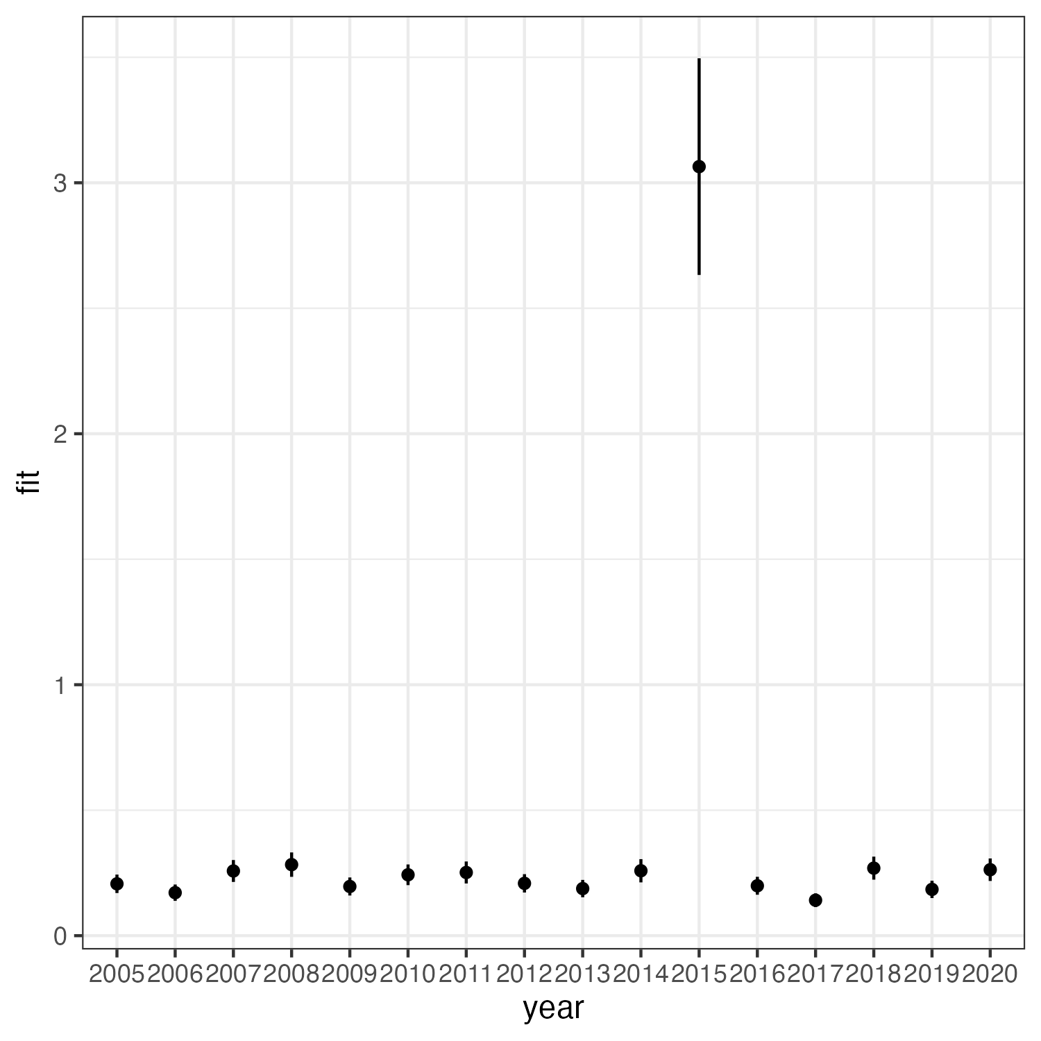
So now in a frequentist framework (I’m familiar with glmmTMB so I use that) I would just fit the model, and get the predictions:
df <- replicated_df %>%
    dplyr::mutate(
        week = as.factor(week),
        year = as.factor(year),
        size = as.factor(site)
    )
freq_mod <- glmmTMB::glmmTMB(
    count ~ year + (1 | week) + (1 | site),
    data = df,
    family = nbinom2
)
predict_data <- data.frame(
    year = as.character(c(2005:2020)),
    week = NA,
    site = NA
)
predicted_yearly <- data.frame(
    year = as.character(c(2005:2020)),
    stats::predict(
        object = freq_mod,
        newdata = predict_data,
        re.form = ~0,
        se.fit = TRUE,
        type = "response"
    )
)
ggplot(predicted_yearly) +
    geom_errorbar(aes(x = year, ymin = fit - se.fit, ymax = fit + se.fit)) +
    geom_point(aes(x = year, y = fit)) +
    theme_bw()
bayes comparison
As far as I understand it for the posterior predictive check, I was following this guide I want to use the tidybayes::epred_draws() function which will operate similarly to stats::predict() (and I assume exactly the same as rstanarm::posterior_predict() but just in a tidy dataframe?
However, herein lies my confusion. For the newdata argument, in the stats::predict() case I would just put NA values for my random effects, set re.form = NA, type = "response" and I get the model-predicted yearly values given my model structure. In this case, I can’t have NA’s in the newdata so you just arbitrarily pick a value for the two random effects that’s actually IN the dataset and use that, then ensure re_formulation = NULL or re.form = NULL and that will give you the conditional means. I’ve tried that here:
# bayesian version of the model
bayes_fit <- rstanarm::stan_glmer(
    count ~ year + (1 | week) + (1 | site),
    data = df,
    family = rstanarm::neg_binomial_2(link = "log"),
    iter = 5000,
    warmup = 2000,
    cores = 4
)

predict_data_bayes <- data.frame(
    year = as.character(c(2005:2020)),
    week = "1",
    site = "one"
)
x <- tidybayes::epred_draws(
    object = bayes_fit,
    newdata = predict_data_bayes,
    re_formula = NULL
)
ggplot(
    x,
    aes(
        x = .epred, y = year, fill = year
    )
) +
    tidybayes::stat_halfeye(.width = 0.95) +
    scale_fill_manual(values = c(rep("lightpink", 16))) +
    labs(
        x = "Count", y = "Year",
        subtitle = "Posterior predictions"
    ) +
    theme(legend.position = "bottom") +
    theme_bw()
Which gives me something like this:

This looks right, but I’m worried I’m confusing something here, and the picking of something arbitrary to go in the newdata feels like I’m doing something wrong and just somehow getting a conditional effect for THOSE specific values not across all random effect levels. Hoping someone can tell me if this is a correct interpretation/implementation of how to move between these two approaches to get what I know is not the SAME thing, but the analogous thing to a model-prediction from a frequentist model.


