Choosing a continuous right skew family for modelling

Hi all,

I am new to brms and Bayesian statistics and am having issues with finding a family to fit my outcome distribution.

I have longitudinal data of depressive symptom ratings from 1-10 across 8 weeks. The daily symptom ratings are summed to form a daily total depression score, which is detrended and scaled across the whole sample and time points. This variable will be referred to as TotalDepression_dt_s for convenience. I am trying to model a simple regression with TotalDepresson_dt_s ~ x + y + z + (1 | PlayerID), with x, y, z, being trait/between-person level variables. Essentially, its attempting to model whether trait predictors are associated with trait/average depression.

The issue I’m having is with finding a good family that matches the distribution of TotalDepresson_dt_s.

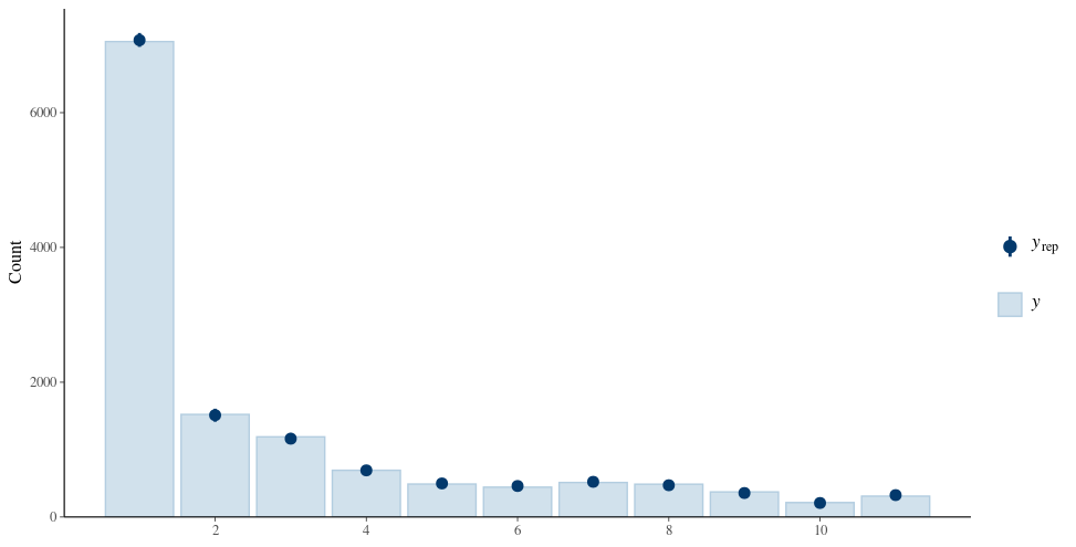
I have tried a gaussian
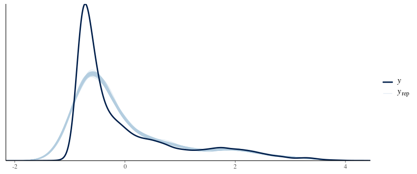

skew_normal

and exgaussian

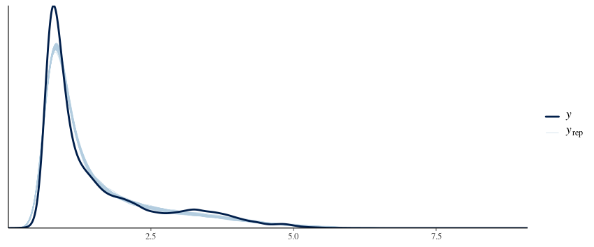
I have also tried shifting the whole distribution to be positive (by adding the min value + 0.001) and fitting lognormal and gamma, which fits similarly well except for the peak. My understanding is that ideally, the family chosen reflects the data generating process-neither of these two families plausibly explains them I think.


I have considered ordinal families (more specifically for the symptom ratings since they reflect the process the best) but there are too many discrete/unique values. The reason is because the data was detrended for each participant by taking the residuals from Depression ~ AssessmentDay + AssessmentDay^(-0.2) and adding it back to the mean, and then scaled across the whole sample. The variables end up losing discrete ordinal categories and becoming continuous (so this issue extends to the individual symptom ratings as well which share a similar distribution).

I have considered a gaussian and skew_normal mixture family but it took forever to run. The issue might be my priors but I don’t think a mixed family is the solution to this problem (happy to be convinced otherwise though).

I wonder if there are any other recommendations on what I should/could do?

1 Like

Hi,
my first guess is that you are looking at artifacts caused by floor effects caused by ordinal nature of the data which then appear smooth due to detrending. I.e. it might be possible to work around this with a suitable distributional family, but that’s fundamentally solving a problem that was created by data preprocessing and is not inherent to the scientific question at hand. For example if there’s a large number of occasions when participants responded close to the lower end of the scale (e.g. had no noticeable depression symptoms).

If you have access to the raw data (which is a big IF), it would IMHO make much more sense to model the ordinal nature of the data (ideally each item of the scale separately) and the trend directly in the same model as you use for your substantial question. My understanding is that things like detrending are hacks that people used because they were not able to fit rich models. These days, you can (usually) fit such models with relative ease - brms specifically will let you model a range of time trend structures.

Note that modelling the “raw” data does not preclude asking questions about the totals/averages or their detrended versions - once the model is fit, you can compute all of those starting from the posterior samples.

Does that make sense?

5 Likes

I second @martinmodrak on this. If possible (and conceptually coherent from your theoretical framework), I’d recommend modeling the original data, rather than detrended scaled version of the data. A good longitudinal ordinal model would probably work remarkably well. Here are a couple posts on the cumulative probit written with psychologists in mind (IDK that you’re a fellow psychologist, but depression items are clearly in our domain):

4 Likes

Also, it looks like this is your first time posting. Welcome to the Stan forums, @pavgreen!

2 Likes

Hi all,

Thank you for the replies and welcome! The advice was really helpful, and I’ve had a read through the recommended readings, though I haven’t had a chance to finish both of them.

If I’m understanding correctly, detrending the model online (by including time as a covariate) instead of offline would allow me to fit an appropriate ordinal family on the data. I’ve fit a quick model predicting one of the symptoms with cumulative(“probit”)

Anxious ~ v + a + ter + v_bias + a_bias + m_bias + v_ratio + age_s + gender + Education + s(AssessmentDay) + (1 | PlayerID)

and it seems to work very well! Importantly, the coefficients match the significance and direction of the frequentist (non-ordinal) approach.

pp_check(bayes_param, ndraws = 1000, type = "bars", prob = 0.95)
pp_check(bayes_param, type = "stat_2d", stat = c("mean", "sd"), ndraws = 1000)


I suppose a follow-up to this is

  1. How do I get the parameter values for “Total Depression” from the posterior?
  2. How would modelling this for a longitudinal REWB model look like?

For 1, I’d assume you’d start off by modelling a multivariate model

bf(mvbind(Lack_of_Interest, Lack_of_Enjoyment, Slow, Tired, Anxious, Worried, Sad, Guilty, Restless, Trouble_Concentrating, Worthless, Irritated, Indecisive, Stressed) ~ v + a + ter + v_bias + a_bias + m_bias + v_ratio + age_s + gender + Education + s(AssessmentDay) + (1 |p| PlayerID))

then maybe extract the relevant posterior parameters and average them? or just model the total as a latent?

With regards to 2, I have a couple of frequentist cross-lagged models that look at confidence_ratings ~ depression and the reverse. The ratings are on a scale of 1-6 and is assessed across 40 trials in a day. In my frequentist model, I’ve simply averaged their confidence ratings to get an average confidence for that specific day’s session and model the association as

confidence_rating_avg_t ~ depression_wpc_t + confidence_wpc_t-1 + depression_mean + (1 | PlayerID)

The model tests for within-person associations in depression (deviations from the mean) and confidence, and trait level depression and confidence, while controlling for within-person autocorrelation of confidence. How would one do this with ordinal data?

Keeping the outcome ordinal should be simple enough if you use raw confidence estimated trials and additionally include AssessmentDay as a random effect. I’d imagine you would similarly average the predictors across all time points to get the between person association.

But what about the within-person associations? What would deviations from a mean for ordinal predictors look like (since you cant have negative values)?

Thank you for the help!

Are the elements in your mvbind() code (e.g., Lack_of_Interest, Lack_of_Enjoyment) the individual Likert-type items?

Yes. They’re rated from 0-10 and are summed to form total depression scores.

Okay. Then instead of fitting a multivariate model with mvbind(), I recommend you put the data in the long format with respect to the depression items and fit them in a multilevel IRT model, such as I did in the blog posts linked above, and as Paul did in his IRT paper: [1905.09501] Bayesian Item Response Modeling in R with brms and Stan. Forgetting time structure and predictors for the moment, that would mean you have a model of the basic form

brm(
  likert_rating ~ 1 + (1 | person) + (1 | item),
  ...
)

You can (and perhaps should) generalize to allow the thresholds to vary by item like so

brm(
  likert_rating | thres(gr = item) ~ 1 + (1 | person) + (1 | item),
  ...
)

From there you can post-process the model to express the sum-score metric like I detailed in the blog post above. Once you have these basic versions up and running, you can then add in time structures and/or predictors as desired.

3 Likes

I’ll second that recommendation - fit an IRT measurement model if possible in this case. Is this a well established measure of depression? If so, you may be able to find good information to inform priors on the item parameters.

1 Like

Thank you for the advice and sorry for the late update, was busy with a conference. I’ve finally managed to read the blog posts and it was really informative.

I currently have issues with fitting lf(0 + (1 | PlayerID) + (1 | Items)) as I’m getting rows of these errors for all chains

...
Chain 4 Rejecting initial value:
Chain 4   Log probability evaluates to log(0), i.e. negative infinity.
Chain 4   Stan can't start sampling from this initial value.
Warning: Chain 4 finished unexpectedly!

Warning: All chains finished unexpectedly! Use the $output(chain_id) method for more information.

Warning: Use read_cmdstan_csv() to read the results of the failed chains.
Warning: No chains finished successfully. Unable to retrieve the fit.
Error: Fitting failed. Unable to retrieve the metadata.

My guess is there’s not enough variation to warrant a different disc parameter for each participant and item. I figure this makes sense given that we’re looking at a general population sample. Running the model without lf seems to work but it takes a very long time, ~ 3 days.

options(mc.cores = 4, brms.backend = "cmdstanr")
control = list(adapt_delta = 0.999)
fam <- cumulative("probit")

prior <- c(prior(student_t(3, 0, 2.5), class = "Intercept"),
           prior(exponential(1), class = "sd"))

bayes_param <- brm(bf(ratings | thres(gr = Items) ~ 1 + (1 | PlayerID) + (1 | Items)), 
                   data = data.IRT, 
                   family = fam, 
                   chains = chains, iter = iter, warmup = warmup, 
                   control = control,
                   threads = threading(threads = floor(parallel::detectCores() / 4)),
                   save_pars = save_pars(all = TRUE),
                   prior = prior)

I wonder if there’s model misspecification which is causing this slowdown? Or is it just the size of the data (186018 rows of data - 162 participants with 14 items across multiple days)? I tried running the model with just 10 participants and it unsurprisingly converges a lot faster.

1 Like