Challenges with se() in meta-analysis

[PritchardAJP]

Hello all,

I am implementing a meta-analysis. My problem is that utilizing the se(sigma=FALSE) seems to be undermining the estimation of the intercept. That is, my intercept gets constrained.

My questions are:
What is going on with the se() parameter? There is no prior to adjust for the se(). I tried adjusting the gaussian identity link, but I do not think that is relevant for as the se() is not a predictor (and its change did not make a difference). Is there anything I can do to fix this beyond adding sigma?

My understanding is that including a parameter for sigma undermines my capacity to interpret the intercept as an average effect size across studies. If I include sigma, and add a formula for it (say: sigma ~ 1 + (1|Group) + (1|Study)), can I still interpret the intercept as average effect size? Note that I have a few other random effects in these data (like Study), that I omitted here for brevity. I am not strictly interested in study differences, because of a few other subgroupings in these data.

---

Here are various forms of my models, trying to isolate the issue

> formula(fit22)
Outcome | se(Se) ~ 1 
> formula(fit23)
Outcome | se(Se) ~ 1 + (1 | Group) 
> formula(fit24)
Outcome ~ 1 
> formula(fit25)
Outcome | se(Se, sigma = TRUE) ~ 1 

You can see (below) that the se() term is the problematic model component (fit22, fit23), which is resolved with its omission (fit24) or the inclusion of a sigma parameter (fit25). Without these changes, the intercept is constrained (thin density) and off-center.

At first I thought it was the default student intercept prior that was the issue, but that is not the case as these runs are with an intercept prior of normal(0, 1.5). Here is the intercept estimate for the fit22 model:

          Estimate Est.Error l-95% CI u-95% CI Rhat Bulk_ESS Tail_ESS
Intercept    -0.03      0.00    -0.03    -0.03 1.00      582      746

The addition of the random effect with the se() term (fit23) does some odd things with intercept convergence.

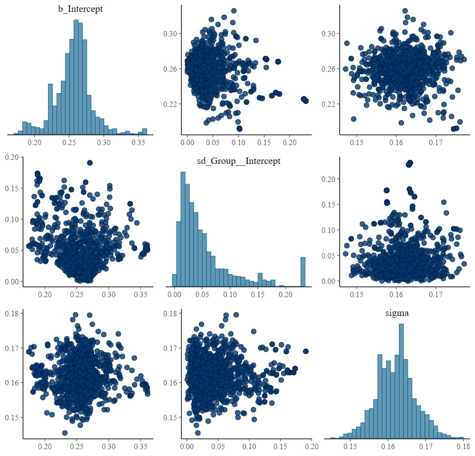
Here is that fit23 pairs plot:

Again, these issues are mitigated (but not fully resolved [I have other random effects that will likely help]) with the addition of the sigma parameter:

> formula(fit26)
Outcome | se(Se, sigma = TRUE) ~ 1 + (1 | Group) 

I do not see any major issue with the distribution of the se() (below), but it is hard to state that definitively without knowing how the model incorporates se(). Note the ‘outlier’ around 0.6 - though I do not think that is the issue.

---

[PritchardAJP]

Though I have not resolved everything, I have improved things slightly. Reconsidering the pp_checks made me concerned that the prior was constraining the posterior. I expanded the prior to normal (0,15).

I think my original priors would have been reasonable with just the Outcome, but the se() must require weaker priors.

Certainly the shape is improved, but I am unsure why the fit is still underestimating the mean. I will play around with things some more, but thought I would share an update should anyone ever see this and have a similar issue.

[PritchardAJP]

This is resolved. The estimation of error for the se() variable is coupled to the actual effect size. This is such that the se shrinks as the effect size approaches 0. In some ways this is logical, but I believe it is strong enough to ‘pull’ the density towards 0 as those estimates are ‘more certain’.

I do not have a modelling solution for this; so, if anyone reads this and has a clever idea, I would appreciate it. Otherwise, I will have to tinker with my se calculations - which is obviously not ideal.

[jsocolar]

I can’t tell for sure whether your explanation corresponds to what is happening here or not, but here is a re-statement of the issue, and below is some code that might help clarify things.

When we don’t estimate a residual standard deviation, one (or a handful of) observations with very tight standard error can pull the estimates around dramatically, regardless of where the rest of the data lands. That’s because the fitted regression had better fit points with small standard errors very well, or incur huge likelihood penalties. The modeling decision that you need to make is: Do you believe that the linear predictor in your regression gives the true values exactly, and that the previous studies have yielded Gaussian uncertainty with accurately quantified standard error, such that all residual variation should be attributed to the standard error? Or do you think there are other sources of stochastic variation, such that there is some residual variation between studies that is not simply inherent in the Gaussian approximations to the posteriors of the study-specific effects? In the latter case, you probably want to include a residual in your model.

library(brms)

#### This model/dataset shows your issue
se_data_1 <- data.frame(
  out = c(3, rnorm(99)),
  se = c(.01, rep(1, 99))
)

mod_1 <- brms::brm(
  out | se(se) ~ 1,
  data = se_data_1,
  backend = "cmdstanr"
)

pp_check(mod_1)

#### This dataset doesn't show your issue
se_data_2 <- data.frame(
  out = c(3, rnorm(99)),
  se = c(rep(1, 100))
)

mod_2 <- brms::brm(
  out | se(se) ~ 1,
  data = se_data_2,
  backend = "cmdstanr"
)

pp_check(mod_2)

[PritchardAJP]

Thanks @jsocolar!

Yes, your example does seem to correspond with what is happening. A lot of posts on meta-analysis suggested to not compute a residual, so I think I was hesitant to do so. That said, for a variety of reasons, I do not really think all the residual variation is attributed to the standard error. So, as long as I am not committing an egregious error, I have no issue with including sigma = TRUE. Other resources seem to suggest that this alters my interpretation of the intercept. I fail to see how this is so, as the model fit seems improved with sigma - why would I trust the intercept of a poorly fit model over the intercept from a model with the residual?