Categorical_logit fitting problem

I tag here @Francesco_De_Vincentis because we are working with an ordinal regression and I noticed a strange behavior.
Let’s say we generate some data with the following model that simulates a regression with only a set of relevant variables:

data {
    int<lower = 0> N;  // number of observation
    int<lower = 0> M;  // number of predictors
    int<lower = 1> K;  // number of ordinal categories
    vector[K-1] c;     // cut points

}

transformed data {
    real<lower = 0, upper = 1> sig_prob = 0.05;
    
}
generated quantities {
    vector[M] beta; // slopes
    matrix[N, M] X; // predictors
    vector[N] mu;
    int y[N];
    
    for (m in 1:M) {
        if (bernoulli_rng(sig_prob)) {
            if (bernoulli_rng(0.5)) {
                beta[m] = normal_rng(10, 1);
            } else {
                beta[m] = normal_rng(-10, 1);
            }
            
        } else {
            beta[m] = normal_rng(0, 0.25);
        }

    }
    
    for (n in 1:N) {
        for (m in 1:M) {
             X[n, m] = std_normal_rng(); // all predictors are mean centered and standardized
        }
    }
    
    mu = X * beta;
    
    for (n in 1:N) {
        y[n] = ordered_logistic_rng(mu[n], c);
    }
}

The parameters are fixed to

set.seed(123)
N = 56 # number of observations
M =  45 # number of predictors
K =   3 # number of ordinal categories

c = sort(runif(n = K - 1, min = -5, max = 5))

The generated slopes are the following:

 [1]  -0.233045611  -0.082993293   0.085635290  -0.135351220  -0.469997342
 [6]   9.353118990   0.412084392   0.062155729   0.128925395   0.037598942
[11]   0.301502594   0.002788009  -0.075224657  -0.143522047   0.123930052
[16]   0.288065551   0.029104101  -0.023312894  -0.040097277  -0.174772110
[21]   9.476527099   0.008296223  -0.297025240  -0.221369662  -0.020534234
[26]   8.771793267 -12.259626932   0.456705693   0.185068152  -0.180819679
[31]  -0.357336895   0.420012002  -0.048720008  -0.209211015  -0.014869948
[36]  -0.237610720  -0.132745718   0.351899836  -0.151526916  -0.092970176
[41]   0.155793645  -0.210137725  -9.580069168  -0.413445021   0.067125648

then, I try to recover the parameters with the following model with very weak priors:

data {
    int<lower = 0> N;           // number of observation
    int<lower = 0> M;           // number of predictors
    int<lower = 1> K;           // number of ordinal categories
    int<lower=1, upper=K> y[N]; // Observed ordinals
    matrix[N, M] X;             // predictors

}

parameters {
    vector[M] beta; // slopes
    ordered[K-1] c; // cut points
    
}

transformed parameters {
    vector[N] mu = X * beta;
}

model {
    c ~ std_normal();
    beta ~ std_normal();
    y ~ ordered_logistic(mu, c);
}

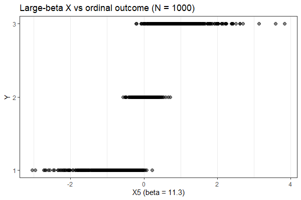
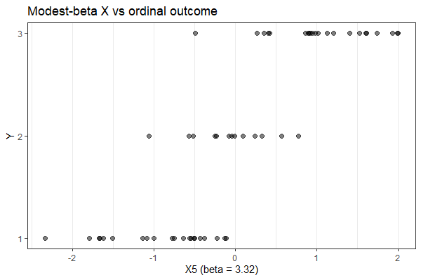
No fitting issues, but the retrieved betas are completely out-of scale:

 [1]  0.55765983 -0.31872757 -0.01912787 -1.03558772 -0.11695698  1.61702316
 [7] -0.16970714 -0.62116552  0.50572192  0.71391765  0.27750075 -0.42554441
[13] -0.15103297  0.30285230 -0.23127667 -0.08122528  1.20845964  0.47454160
[19] -0.48673457  0.67766070  1.47488536 -0.34840871 -0.93800531 -0.01341664
[25]  0.04542973  1.40791297 -2.13944193  0.28727535  0.33961248  0.65462492
[31] -0.08853437  0.35295322 -0.68077223 -0.47923495 -0.49212390 -0.25563038
[37]  0.38995377 -0.07001296 -0.86405367  0.21519595  0.24711355 -1.01672975
[43] -1.80061339 -0.30204615 -0.02697607

what am I doing wrong?

I don’t think the std_normal would class as a weak prior here at all. Your cutpoints are generated uniformly between -5 and 5, but the N(0,1) prior has ~99.9% of its density between -3 and 3. Similarly some of your coefficients are as large as 9 - 12, which the N(0,1) prior implies is extremely unlikely

1 Like

@andrjohns yep! exactly? Are there some flatter priors to try? any advice?

What happens if you use a wider prior, like the default uniform? At the very least you’ll need a larger scale parameter for the normal, like a normal(0,5) or similar

If you’re trying to recover generated parameters then your priors need to match, or at least cover the parameters used to generate the data. If some of your beta coefficients were generated using a normal(10,1) distribution, then it’s very unlikely that a normal(0,1) prior will recover that. Same for the cutpoints, if they’re generated using a uniform(-5, 5) distribution, then a normal(0,1) prior could struggle.

1 Like

@andrjohns I understand. I tried to decouple as much as possible the generative process and the fitting model. This is because we’ll work on real data where we do not know where the cutpoints are and the magnitude of the betas is unknown…
However… I will try with flatter priors and I will tell you how it goes!

1 Like

Alongside @andrjohns 's excellent advice, I would consider whether your DGP parameters are realistic to the problem you have in mind, as I believe that they are making the estimation problem much more challenging than they may need to be. Most specifically, betas of \pm10 and cutoffs around \pm2 generate large areas of non-overlap, which can make ordinal models unstable.

I generated the data according to your DGP and estimated your target model. Notice in the plot below that there is no overlap on X5 for respondents where Y=1 and Y=3 And in the second plot below, you can see that the large coefficient (X5) is nearly 3 times larger than its estimate.

x-y overlap

dgp vs target big beta

There are 3 solutions I can think of.

  1. Generate larger samples to better estimate that overlap
  2. Reduce the size of the large effects to increase the overlap
  3. Use something like a horseshoe prior to pick out the large betas and shrink the small ones

By increasing your sample size, you can better estimate the overlap on the large-coefficient dimension, which helps stabilize the ordinal model.

x-y overlap large n

dgp vs target large n

By using a smaller large signal, you also increase the overlap though without increasing the sample size. Would it still be realistic if you changed \pm10 to \pm2, as was used in the DGP below?

x-y overlap2

dgp vs target modest beta

Given your DGP is made up of a few large signals and many very small signals, a horseshoe prior seems appropriate. It certainly looks better than the standard normal from a signal detection standpoint, though it is less clear to me whether this would work well across different repetitions. Here are the beta estimates when the large beta distributions are centered at \pm10.

beta horseshoe

I just mixed the advice of @simonbrauer and @andrjohns : flatter priors on c and horseshoe priors on \beta have done the trick!
Thanks in advance!