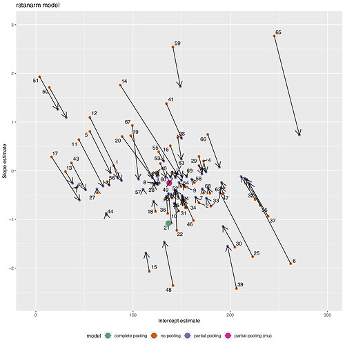
Can partial pooling lead to shrinkage in multiple directions?

I am building a model with partial pooling, but noticed that some estimates are not being pulled directly to the population-average, and more off to one side. I found this same response to also occur when using test data. Is it possible for models with partial pooling to not always pull directly towards the same point? Does this suggest an issue with my model formatting? Or is it normal, and likely driven by differences in the variance across groups?

For context, I am building a model to analyze long-term data of species life history events (day of flowering, egg laying, reproduction, etc.). Each data point represents the day the event occurred for a given year of observation, but there is high diversity in the species included, type of events, and the length of each observation period can range from 5-30 years. I am primarily interested in seeing how the species slopes are changing over time. To do this, I have been developing a model with random slopes and intercepts and partial pooling for different species. To plot the extent of the partial pooling, I used the vignette found here.

My Stan code is the following:


data {
  int<lower=0> N; //No. observations
  int<lower=0> Nspp; //No. species
  int species[N]; // Grouping by species
  vector[N] year;
//response
  real ypred[N]; //day of year for nat. history event
}

parameters {
  real a[Nspp] ;// intercept for species 
  real b[Nspp]; // slopes for species

  real mu_a; //mean int across sp 
  real<lower=0> sigma_a; // variation in intercept among species
  real mu_b; // mean slope across sp
  real<lower=0> sigma_b; //var of slope among sp

  real<lower=0> sigma_y; //measurement error 
  
}

transformed parameters{
  real mu_y[N]; //individual mean

  for(i in 1:N){
    mu_y[i]=a[species[i]]+b[species[i]]*year[i];
  }
}

model {
  a ~ normal(mu_a, sigma_a);
  b ~ normal(mu_b, sigma_b);

    //Priors
  mu_a ~normal(188, 50); 
  sigma_a ~normal(0,50);
  mu_b ~normal(0,10); 
  sigma_b ~normal(0,10); 
  sigma_y ~normal(0,10); 

  ypred ~ normal(mu_y, sigma_y);
  
}

I would really appreciate any clarification as to whether such observed trends are to be expected given the type of data I am working with or if there are ways I should be adjusting the model itself.

Thanks!

1 Like

@betanalpha @andrewgelman @jonah

OK, a bunch of quick comments:

  • With multiple parameters, partial pooling can indeed do unexpected things sometimes. The prior for the intercept in a regression will affect what happens to the slope.
  • I could comment on the Stan model, but I think it would make sense to write the above model in rstanarm or brms rather than Stan. Using a wrapper such as rstanarm or brms would allow you to focus on the modeling, then you could always go into Stan if needed later.
3 Likes

Thanks @maxbiostat for bringing this to others attention!

Thank you @andrewgelman for taking the time to comment!

I will take your suggestion and try writing the model using rstanarm or brms and see if I get similar shrinkage.

Thanks @maxbiostat and @andrewgelman It’s a great idea to check out code against rstanarm or brms (I just like rstan for its readability and flexibility).

I have often seen partial pooling do weird stuff with multiple parameters. See for example the plot below – this one made sense as we had three partially pooled slopes in the model and were looking at just one.

In @Deirdre_L plots it’s overshooting the complete pooling and \mu from the partial pooling, but there are not really other parameters to cause this, in my mind at least (\sigma_y?) so it’s seems very odd.

@Deirdre_L if you cannot solve this through troubleshooting a small dataset in rstanarm versus your rstan code, maybe you can show one of the plots I was looking at.

I’d just like to understand what’s going on before pushing ahead on the model.

Thank you again @andrewgelman for your suggestion to focus on the modeling with rstanarm.

In doing so, the output was essentially the same, and I continued to get the same shrinkage for some of my species. In particular, I am concerned about the shrinkage for the cluster of species that includes 6, 32,35,37 (located around (230, -0.5)), species 17 (20, 0.4), and species 65 (245, 2.9).

I have included the rstanarm model I used and the code and data to make the above plot:

synch_datasub_sd.csv (50.7 KB)


# rstanarm model
synch<-stan_lmer(formula = doy ~ yr1980 + (1 + yr1980 | species.fact), data =synchdat)

# making the plot as per T. Mahr’s vignette 

com.pool.mod <- lm(doy ~ yr1980, synchdat)
spp <- sort(unique(synchdat$species.fact))
no.pool <- data.frame(species=rep(NA, length(spp)),
                    intercept=rep(NA, length(spp)), 
                      yr1980=rep(NA, length(spp)) 
)

df.gravity <- no.pool[1:2,2:3]
no.pool$model <- "no pooling"

#no pooling
for (sp in c(1:length(spp))){
  no.pool$species[sp] <- spp[sp]
  subby <- subset(synchdat,  species.fact==spp[sp])
  lmfit <- lm(doy ~ yr1980, data=subby)
  no.pool$intercept[sp] <- coef(lmfit)["(Intercept)"]
  no.pool$yr1980[sp] <- coef(lmfit)["yr1980"]
}

#parital pooling 
with.pool<-coef(synch)[[1]]
names(with.pool)[names(with.pool) == '(Intercept)'] <- "intercept"
with.pool$model <- "partial pooling"
head(with.pool)

no.pool$species <- sort(unique(synchdat$species.fact))
with.pool$species <- sort(unique(synchdat$species.fact)); with.pool<-with.pool[,c(1:4)]
df.pulled <- rbind(no.pool, with.pool)

head(df.pulled)

df.gravity$model <- NA
df.gravity$intercept[1] <-coef(com.pool.mod)["(Intercept)"]
df.gravity$yr1980[1] <-coef(com.pool.mod)["yr1980"]
df.gravity$model[1] <- "complete pooling"
df.gravity$intercept[2] <- synch$coefficients[1]
df.gravity$yr1980[2] <- synch$coefficients[2]
df.gravity$model[2] <- "partial pooling (mu)"

ggplot(df.pulled) + 
  aes(x = intercept, y = yr1980, color = model) + 
  geom_point(size = 2) + 
  xlim (-5,300) + ylim (-2.6,3) + 
  geom_point(data = df.gravity, size = 5) + 
  # Draw an arrow connecting the observations between models
  geom_path(aes(group = as.character(species), color = NULL), 
            arrow = arrow(length = unit(.02, "npc"))) + 
  # Use ggrepel to jitter the labels away from the points
  ggrepel::geom_text_repel(
    aes(label = species, color = NULL),
    data = no.pool, size=4) +
  theme(legend.position = "bottom") + 
  ggtitle("rstanarm model") + 
  xlab("Intercept estimate") + 
  ylab("Slope estimate") + 
  scale_color_brewer(palette = "Dark2") 


Any insights into what could be driving these trends or suggestions for what I could explore next would be greatly appreciated.

Thanks!

@Deirdre_L My guess is it’s the covariance matrix … as there isn’t much else it could be and you got the same output in rstanarm. I just can’t see through quickly how to extract it (in rstanarm) and check that it’s causing the observed behavior. Though I guess as a quick check you could plot the intercepts versus slopes and see where these species show up?

If others have guesses – or suggestions on how to check if it’s the covariance matrix – please toss 'em out there.

Thanks!
Lizzie

One complication with hierarchical models is that everything is uncertain, including not just the individual parameters but also the population parameters that control the partial pooling. The joint posterior between the individual parameters and the population parameters can exhibit strong degeneracies that result in odd behavior in any point estimates, especially means when those degeneracies are skewed. For example while the point estimate of the pooled individual parameters might look odd the full posteriors for the baseline and the individual parameters might actually overlap!

1 Like