Ok, success! I estimated a multilevel model for a (r \times t \times s) G study, which means I needed random intercepts for r, t, s, r:t, r:s, and t:s. I ended up using informative cauchy() priors on the SD parameters and an informative normal() prior on the intercept.
library(tidyverse)
library(brms)
library(tidybayes)

bgt <-
  brm(
    formula = bf(rating ~ (1 | rater_id) + (1 | target_id) + (1 | condition) +
      (1 | rater_id:target_id) + (1 | rater_id:stimulus_type) +
      (1 | target_id:stimulus_type)),
    prior = c(...),
    data = dat,
    ...
  )
Then, for each posterior draw, I needed to pull out the intercept for each SD parameter and square it to get the variance estimate. These estimates could then be summed to calculate the total variance and then the proportion of the total variance explained by each. Finally, I summarized across all draws by calculating the posterior medians and highest density continuous intervals.
bgt %>%
  tidy_draws() %>%
  select(starts_with("sd_"), sigma) %>%
  transmute_all(.funs = list(sq = ~(. ^ 2))) %>%
  mutate(total_var = rowSums(.)) %>%
  mutate_at(.vars = vars(-total_var),
            .funs = list(pct = ~(. / total_var))) %>%
  map_df(.f = ~ median_hdci(., .width = 0.95), .id = "component") %>%
  mutate(
    component = str_remove(component, "sd_"),
    component = str_remove(component, "__Intercept_sq"),
    component = str_replace(component, "sigma_sq", "residual")
  )
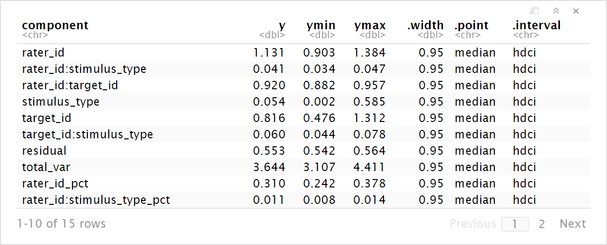

These estimates are quite similar to the REML ones I got from a frequentist G study, but have the added benefits of including interval estimates and avoiding negative variance estimates.