I am using brms to fit a model with nested clustering (i.e., each target is rated by each rater):
  brm(
    formula = rating ~ 1 + x1 + x2 + x3 + (1 | rater / target),
    prior = c(...),
    data = data
  )
If possible, I would like to quantify how much of the variance in rating was explained by each of the predictors: x1, x2, and x3 as well as by the clustering variables rater and target. I get the sense from searching here that the key may be using posterior_linpred() or posterior_predict() but I’m hoping someone can confirm this. Also, would it change things if I had interaction effects and/or random slopes?
An explanation would be ideal, but relevant references would also be appreciated. Thanks!
This problem has no proper answer if the terms are correlated with each other as, in this case, there is no unique way to assign variance explained to predictors separately (in general).
Are you directly interested in the varianeces explained or do you have some other goal which you just try to answer by means of variances explained?
Rights, J.D., & Sterba, S.K. (in press). Quantifying explained variance in multilevel models: An integrative framework for defining R-squared measures. Psychological Methods.
But if that’s not possible, perhaps you could help me achieve a similar goal: (1) How much variance was explained by each clustering variable: rater and target? (2) How important was each predictor?
For (1), perhaps performance::icc() is relevant. I get this output but am not fully sure how to interpret it. This also doesn’t seem to separate out the two clustering variables (perhaps this isn’t possible).
# Random Effect Variances and ICC

Conditioned on: all random effects

## Variance Ratio (comparable to ICC)
Ratio: 0.77  CI 95%: [0.76 0.78]

## Variances of Posterior Predicted Distribution
Conditioned on fixed effects: 0.81  CI 95%: [0.77 0.84]
Conditioned on rand. effects: 3.47  CI 95%: [3.42 3.52]

## Difference in Variances
Difference: 2.66  CI 95%: [2.60 2.72]
For (2), I guess I can interpret the regression coefficients but I’d like (if possible) to be able to compare the “importance” of the predictors to that of the clustering variables. Explained variance seemed like a possible approach to this, but maybe I’m not thinking this through enough.
Thanks for helping me work through this. This community is great.
I’ve been reading a lot more about frequentist and Bayesian approaches to Generalizability theory and found the following papers very informative:
Jiang, Z. (2018). Using the Linear Mixed-Effect Model Framework to Estimate Generalizability Variance Components in R. Methodology , 14 (3), 133–142. https://doi.org/10/gfxf43
LoPilato, A. C., Carter, N. T., & Wang, M. (2015). Updating Generalizability Theory in Management Research: Bayesian Estimation of Variance Components. Journal of Management , 41 (2), 692–717. https://doi.org/10/gcp2sf
Based on this, it looks like I should reformulate my model to focus on sources of variance:
Then I should be able to derive the variance component for each source from the posterior draws and calculate the desired Generalizability coefficients. Will follow up once my model converges and I can play with this some more.
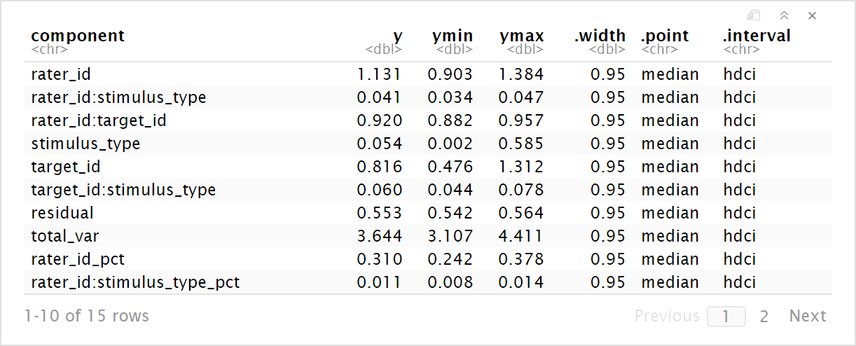
Ok, success! I estimated a multilevel model for a (r \times t \times s) G study, which means I needed random intercepts for r, t, s, r:t, r:s, and t:s. I ended up using informative cauchy() priors on the SD parameters and an informative normal() prior on the intercept.
Then, for each posterior draw, I needed to pull out the intercept for each SD parameter and square it to get the variance estimate. These estimates could then be summed to calculate the total variance and then the proportion of the total variance explained by each. Finally, I summarized across all draws by calculating the posterior medians and highest density continuous intervals.
These estimates are quite similar to the REML ones I got from a frequentist G study, but have the added benefits of including interval estimates and avoiding negative variance estimates.
Also, based on ten Hove et al. (2020), I switched from half cauchy to half student_t priors on the intercept SD parameters, switched from the posterior median to the posterior mode for point estimates, and added random inits.