I have a question about valid distributions in Stan with two parts:
About fabs()
Section 3.7. of the function reference manual lists Step-like functions with a warning saying that the functions listed there break gradients. I understand that is the case regarding all the functions except fabs().
Why would fabs() breaks gradients? I guess that one hard requirement is that the function would be differentiable, which unless I’m very wrong fabs is fine. And another softer requirement is that the function doesn’t have funnels or narrow areas, right? Not sure what is the mathematical name for that.
It’s also confusing to me that the Example 19.1 in the User Manual is about creating a custom distribution with fabs(). So my question is, is fabs() problematic, if so why?
The double monomial distribution
I found an obscure distribution, and I’d like to know if it’s potentially problematic for Stan. I wrote the code of its PDF below in R, and some plot. It’s differentiable, but it has an elbow at t_0 (like fabs()) is this a problem? (If so why?)
Someone smarter will have to answer that one (maybe @nhuurre).
My guess is that it may just be less likely to cause issues for the sampler, but it still might? I mean the gradient is till undefined for x = 0 (x/(x^2 - abs(x))).
I also know this is used to the triangle distribution example in the Stan User Guide which is why I fear I may be missing something.
It’s not, or rather, it’s just as bad as fabs() which means it’s kinda-sorta bad but not a disaster.
The problem is that when the integrator steps over the discontinuity (in the derivative) there is an unexpectedly large error in the energy. This forces the integrator to use a smaller step size to achieve the target acceptance rate.
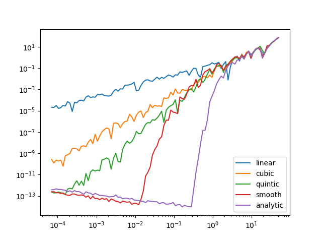
Furthermore, the scaling between acceptance rate and step size changes. Here’s a plot (taken from the interpolation discussion) of the energy error (\approx the probability of rejecting the transition) as a function of step size. “Analytic” is the ideal behavior and “linear” has fabs()-like corners.
I thought that the step size was decided during the warm up and it was fixed, and hence the problem with the funnel in hierarchical models
This is from the user guide:
This is due to the fact that the density’s scale changes with y, so that a step size that works well in the body will be too large for the neck, and a step size that works in the neck will be inefficient in the body. This can be seen in the following plot.
Yes, step size is fixed after adaptation. I meant adaptation adjust step size to meet the target adapt delta.
It’s the same problem: a very small step size is required near the corner even if larger step size should work everywhere else.
The problem is mostly the inefficiency. If you don’t care about runtime then you can sample any distribution with the classic Metropolis-Hastings algorithm, no derivatives needed.
HMC degrades somewhat gracefully, nondifferentiable points mostly just make it behave more like Metropolis-Hastings and not fail completely.
what about distributions like the double monomial distribution, (see the pic above) which has an “elbow”. is it the same issue even if it’s differentiable?
In practice the integrator cannot resolve features much smaller than the step size so how sharp the “elbows” are matters more than whether something is technically differentiable.
Just to add a bit more detail – the dynamic Hamiltonian Monte Carlo sampler used in Stan generates transitions by first creating a numerical Hamiltonian trajectory and then selecting a point from that trajectory based on the Hamiltonian error. If the numerical Hamiltonian trajectory closely matches the exact Hamiltonian trajectory then all points will have reasonably small error and points far away from the initial point will be just as likely to be chosen as points close to the initial point. This is what leads to such effective transitions.
Any non-differentiable cusps in the target density function, however, cause the numerical Hamiltonian trajectory to strongly deviate from the exact Hamiltonian trajectory and any points in the numerical trajectories generated after encountering the cusp will be chosen only with negligible probability. In other words transitions will be limited to only those points generated before encountering the cusps, which tend to be very close to the initial point.
A single point at which the target density is non-differentiable may not sound like a significant problem, but it is. The problem is that the numerical Hamiltonian trajectories need to take the cusp into account not just every time they land on the cusp but rather every time they pass by the cusp. Even if numerical trajectories will never land on the cusp they will pass it often, resulting in the degraded sampling performance.
I’m not sure on what Wolfram Alpha is relying here but that density function absolutely isn’t differentiable at t_{0}. For t < t_{0} the derivative is positive and non-zero while for t > t_{0} the derivative is negative and non-zero. No matter how the density function is define at t_{0} these two behaviors cannot be connected.
If your target density function is defined entirely by this double monomial density function then yes there will be degraded sampling performance, although it might still be high enough to be okay in any given application. If this target density function is being used as a prior model or observational model, however, then the other contributions to the target density function might wash out the cusp or suppress the total target probability around the cusp so that it’s encountered only rarely.
Similar issues arise, for example, with Laplace prior density functions.
It can be both, depending on the severity of the discontinuity and how the parameters configure the shape of the density function.
Even though the discontinuity appears to be one-dimensional in the plots of the observational density it will manifest in a much more complicated discontinuity likelihood function over the parameter space, where the latent parameters may have to move in correlated ways to cross the peak. Each observation will also introduce it’s own discontinuity here the peak passes the observation, and so the total posterior will have lots of discontinuities. This can not only limit how quickly the sampler can move from one part of the typical set to another, it can also prevent sufficient exploring at all.
SBC can definitely help, although if the bias is small the SBC deviations might be hard to resolve without lots of simulations.
I tried reasoning through some behaviors that you could check against but I can’t convince myself if they’d actually work or not. Mathematically the discontinuities will always be there, but the posterior distribution might concentrate sufficiently far away from from the discontinuities that their effects are negligible (like suppressing undesired modes with a strong prior model --they never actually go away, you just make them small enough to be negligible). The challenge is figuring out where the discontinues in the parameter space arise and then comparing that to the posterior, which is nontrivial.