Bayes factors for a series of experiments using posteriors as priors

Hey all,

I’ve a rather conceptual but still specific question for a current project. This question is likely to come up again in my work and I think is quite relevant for my field (psychology/neuroscience) in terms of we how currently collect and present evidence. Therefore and because I want to get this right for a pre-registration of that study, it would be great to get some input.

In sum, I want to provide evidence that an outcome is a quadratic (in fact U-shaped1) function of my predictor. This is my model:

brm(y ~ x + I(x*x) + (1 | subject) + (1 | stimulus)).

There are two cases for which I have the same prediction. In one case the link function is Gaussian and in the second case the link function is Bernoulli.

Our theory predicts that I(x*x) is positive and I want to quantify the evidence for/against that. I’ve already ran three experiments that with the same design and data structure. Unfortunately by the time I’ve started this study, I wasn’t aware of Stan or brms so I’ve analysed the data with frequentist mixed models but the specific hypothesis and predictions were also pre-registered. In that analysis, two out of the three experiments show ‘significant’ quadratic effects. Since I now know that brms exists, I want to re-analyse the data and run a fourth experiment.

My original plan was/is to use the posterior distribution of my beta parameters (intercept, beta1 & beta2) as prior for the subsequent experiments. How is that feasible? How do I have to model the dependency between the betas that this works? I think for me that would be the neatest way for the article that I want to write. Should may use poly() instead of I() that the terms are orthogonal?

I’ve briefly talked to Paul Buerkner during StanCon in Cambridge and he hinted that I could just analyse all experiments in one go but I struggle how I incorporate the random intercepts for subject and stimulus that are nested within the experiments. Is this model

brm(y ~ x + I(x*x) + (x + I(x*x) | experiment) + (1 | subject) + (1 | stimulus))

what I am looking for? If I choose this how do I evaluate the evidence from a future experiments? Do I just re-run the model with this data included? Is that (because of different hierarchical structure) equivalent to using posteriors as priors?

In order to quantify and report the evidence, I know I can just examine the posterior distribution and check whether zero is included in the 95 % credibility interval but for the journal/reviewers are unlikely to accept this but want to see Bayes Factors. How can I use the previous evidence to generate priors for my last experiment? Is it permissible to retroactively choose weakly informative prior or even a super-vague prior as specified here for the analysis for the already existing data?

It would be great if I could feedback on this because it’s my first stan/brms project and I want to do similar things in the future.

1 Here, it could be interesting to model fit two lines based on a breaking point as Simonsohn suggests here but it’s completely over my head and I have no idea how implement this with my data structure in hierarchal Bayesian model.

Between my long-ago Frequentist days and my current Bayesian days, I spent a few years espousing likelihood ratios as endpoints of statistical analyses. With LRs, you could combine evidence from multiple studies by merely multiplying their LRs together. From what I gather BF’s seem very similar to LRs mathematically and philosophically, so is it possible you can simply multiply your BFs?

If you include model 1’s prior as model 2’s posterior, it is the same thing as just combining the data from data1 with data2.
As in:

p(\theta,Y_1,Y_2) = p(Y_2|\theta)p(\theta|Y_1)p(Y_1) = p(Y_1,Y_2|\theta)p(\theta)

So if you’re going to use a posterior as a prior in a second model, you may as well just combine all the data and estimate it in one go.
This will also be the exact same thing as a fixed effects meta-analysis.

Paul’s suggestion includes a random effect of experiment. If there are differences between the experiments in any way, then this would probably be the preferred option. This is akin to a random effects meta-analysis. You assume there can be minor (or major, I guess) differences between the experiments. Then you get a distribution of effects across experiments.

A word of caution: If you run the model you proposed, ensure that subject is unique across all studies; that is, if you have ‘subject 1’ in both experiment 1 and 2, and they are not the same person, then you should have a unique ID for them. Alternatively, you can use (1 | experiment:subject). Likewise with stimulus; if stimulus 1 is different across studies, you should have unique id’s, or tell brms they are nested within experiment using (1 | experiment:stimulus).

Thank you that is really helpful! I think going for a random effect is sensible in terms of getting a better idea of the uncertainty.

However, when I fit the model with experiment as a random effect sometimes I get a small number of transitions after warmup around 5 with (adapt_delta = 0.9999) that I don’t get any if I don’t includes this. How problematic are these in that case?

When I simulate this, I do get different values and different distributions and I am wondering whether that is only noise.
unnamed-chunk-12-1
I described this simulation here, but basically I created two datasets and compared analysing them in one go or sequentially.

My question is whether the observed difference is just noise or a significant bias? I set the post-warm-up samples to 30,000, which I hope to be enough.

At first I thought, using normal priors was the probIem but I still get a shift to the right for the sequential analysis if I fit a student distribution to capture the posterior distribution of model 1 (see script).

Am I missing something here?

Sorry for bumping this topic up but I recently visited the question. I’ve simulated an extremely simple example and found that this doesn’t seem to work at all.

My main question is why does this not work? It should right?

So, created two data sets that have slightly different beta-values:

# Libraries
library(brms)
library(assortedRFunctions) # devtools::install_github("JAQuent/assortedRFunctions", upgrade = 'never')
cores2use <- 4
samples_for_priors <- 20000

# Generating data 1
n1      <- 100
beta1.0 <- 0
beta1.1 <- 0.2
x       <- runif(n1, -1, 1)
y       <- beta1.0 + beta1.1*x + rnorm(n1, 0, 1)
data1 <- data.frame(x, y)

# Generating data 2
n2      <- 50
beta2.0 <- 0.2
beta2.1 <- 0.3
x       <- runif(n2, -1, 1)
y       <- beta2.0 + beta2.1*x + rnorm(n2, 0, 1)
data2   <- data.frame(x, y)

# Combining data sets
data_combined <- rbind(data1, data2)

To test whether chucking everything into one model is the same as first analysing data1 and then data2, I combine data1 & data2 into pooled data frame data_combined.

I then run the first model on data1 and fit a student distrubtion to the posterior distribution for each parameter in this model (Intercept, b_x & sigma). These distributional parameters are used to serve as priors for the model on data2. I also run null models by removing b_x so I can compare various ways of calculating the BFs.

# Sequential analysis
# Data 1
initial_priors <- c(prior(normal(0, 1), class = "Intercept"),
                    prior(normal(0, 1), class = "b")) 

initial_prior_null <- c(prior(normal(0, 1), class = "Intercept")) 

m_data1 <- brm(y ~ x, 
               data = data1,
               prior = initial_priors,
               chains = 8,
               warmup = 2000,
               iter   = 26000,
               cores = cores2use,
               save_all_pars = TRUE,
               sample_prior = TRUE)

m_data1_null <- brm(y ~ 1, 
                   data = data1,
                   prior = initial_prior_null,
                   chains = 8,
                   warmup = 2000,
                   iter   = 26000,
                   cores = cores2use,
                   save_all_pars = TRUE,
                   sample_prior = TRUE)

# Getting priors for Data 2
# Full model
# Get posterior
postDists <- posterior_samples(m_data1)
samples   <- nrow(postDists)
postDists <- postDists[sample(samples, samples_for_priors),]

# Fit model to get distribution
b_Intercept <- brm(b_Intercept ~ 1,
                   data = postDists,
                   cores = cores2use,
                   family = student(link = "identity", link_sigma = "log", link_nu = "logm1"))

# Fit model to get distribution
b_x <- brm(b_x~ 1,
           data = postDists,
           cores = cores2use,
           family = student(link = "identity", link_sigma = "log", link_nu = "logm1"))

# Fit model to get distribution
sigma <- brm(sigma ~ 1,
             data = postDists,
             cores = cores2use,
             family = student(link = "identity", link_sigma = "log", link_nu = "logm1"))

# Fit model to get distribution
priors_data2  <- c(set_prior(priorString_student(b_Intercept), 
                             class = "Intercept"),
                   set_prior(priorString_student(b_x), 
                             class = "b", 
                             coef = "x"),
                   set_prior(priorString_student(sigma),
                             class = 'sigma'))

# Null model
# Get posterior
postDists <- posterior_samples(m_data1_null)
samples   <- nrow(postDists)
postDists <- postDists[sample(samples, samples_for_priors),]

# Fit model to get distribution
b_Intercept <- brm(b_Intercept ~ 1,
                   data = postDists,
                   cores = cores2use,
                   family = student(link = "identity", link_sigma = "log", link_nu = "logm1"))

# Fit model to get distribution
sigma <- brm(sigma ~ 1,
             data = postDists,
             cores = cores2use,
             family = student(link = "identity", link_sigma = "log", link_nu = "logm1"))

# Fit model to get distribution
priors_data2_null  <- c(set_prior(priorString_student(b_Intercept), 
                             class = "Intercept"),
                   set_prior(priorString_student(sigma),
                             class = 'sigma'))

# Run full model for data 2
m_data2 <- brm(y ~ x, 
               data = data2,
               prior = priors_data2,
               chains = 8,
               warmup = 2000,
               iter   = 26000,
               cores = cores2use,
               save_all_pars = TRUE,
               sample_prior = TRUE)

# Run null model for data 2
m_data2_null <- brm(y ~ 1, 
               data = data2,
               prior = priors_data2_null,
               chains = 8,
               warmup = 2000,
               iter   = 26000,
               cores = cores2use,
               save_all_pars = TRUE,
               sample_prior = TRUE)

I also run a model on the pooled data that:

# Combined analysis
m_data_combined <- brm(y ~ x, 
                       data = data_combined ,
                       prior = initial_priors,
                       chains = 8,
                       warmup = 2000,
                       iter   = 26000,
                       cores = cores2use,
                       save_all_pars = TRUE,
                       sample_prior = TRUE)


m_data_combined_null <- brm(y ~ 1, 
                            data = data_combined ,
                            prior = initial_prior_null,
                            chains = 8,
                            warmup = 2000,
                            iter   = 26000,
                            cores = cores2use,
                            save_all_pars = TRUE,
                            sample_prior = TRUE)

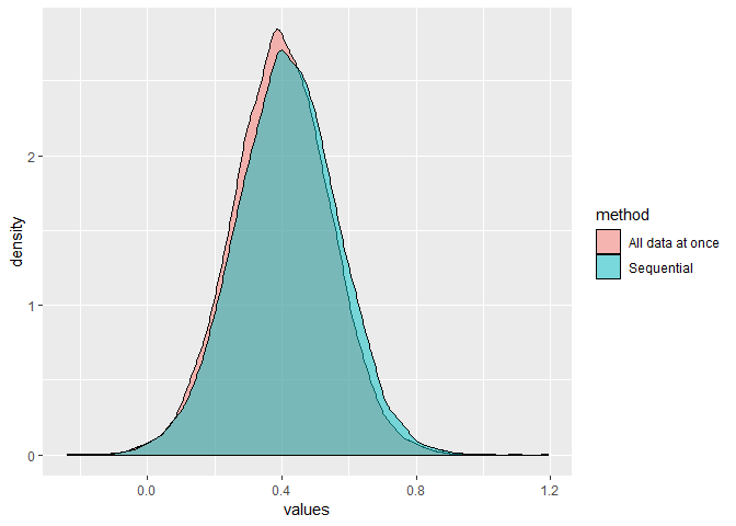
If I compare the posterior distributions for Intercept & b_x from m_data2 and m_data_combined, I see that the distribution seems to be quite different. I used a lot of samples on purpose but it seems very robust.
Look at the difference for the Intercept

and for b_x

This difference is also evidence in the BFs that I calculate in three (two using Savage Dickey ratio & one using bayes_factor()) ways:

# Method: hypothesis()
# Data 1
bf_hypo_1      <- 1/hypothesis(m_data1, 'x = 0')$hypothesis$Evid.Ratio

# Data 2
bf_hypo_2      <- 1/hypothesis(m_data2, 'x = 0')$hypothesis$Evid.Ratio

# Pooled
bf_hypo_pooled <- 1/hypothesis(m_data_combined, 'x = 0')$hypothesis$Evid.Ratio

# Method: Manual with logspline
library(polspline)
# Data 1
priorDist    <- prior_samples(m_data1)$b
fit.prior    <- logspline(priorDist)
priorDensity <- dlogspline(0, fit.prior)

postDist      <- posterior_samples(m_data1)$b_x
fit.posterior <- logspline(postDist)
posterior     <- dlogspline(0, fit.posterior)
bf_manual_1   <- priorDensity/posterior

# Data 2
priorDist    <- prior_samples(m_data2)$b
fit.prior    <- logspline(priorDist)
priorDensity <- dlogspline(0, fit.prior)

postDist      <- posterior_samples(m_data2)$b_x
fit.posterior <- logspline(postDist)
posterior     <- dlogspline(0, fit.posterior)
bf_manual_2   <- priorDensity/posterior

# Pooled
priorDist    <- prior_samples(m_data_combined)$b
fit.prior    <- logspline(priorDist)
priorDensity <- dlogspline(0, fit.prior)

postDist         <- posterior_samples(m_data_combined)$b_x
fit.posterior    <- logspline(postDist)
posterior        <- dlogspline(0, fit.posterior)
bf_manual_pooled <- priorDensity/posterior

# Method: bayes_factor()
# Data 1
bf_bayes_factor_1 <- bayes_factor(m_data1, m_data1_null)

# Data 2
bf_bayes_factor_2 <- bayes_factor(m_data2, m_data2_null)

# Pooled
bf_bayes_factor_pooled <- bayes_factor(m_data_combined, m_data_combined_null)

For higher BFs the results acutally often give quite different estimates but for smaller beta they are pretty much in agreement.

BFs from method 1

Approach data1 data2 combined
sequential 1.97189005763761 0.875614188723706 1.726615
combined 3.027281

BFs from method 2

Approach data1 data2 combined
sequential 2.02109969356174 0.828254520749124 1.673985
combined 3.155711

BFs from method 3

Approach data1 data2 combined
sequential 2.01844391362641 0.755140228408023 1.524208
combined 3.088728

Conclusion

I am extremely confused and would love to have some comment on this.

sessionInfo():

R version 3.6.2 (2019-12-12)
Platform: x86_64-w64-mingw32/x64 (64-bit)
Running under: Windows 10 x64 (build 17763)

Matrix products: default

locale:
[1] LC_COLLATE=English_United Kingdom.1252  LC_CTYPE=English_United Kingdom.1252    LC_MONETARY=English_United Kingdom.1252
[4] LC_NUMERIC=C                            LC_TIME=English_United Kingdom.1252    

attached base packages:
[1] stats     graphics  grDevices utils     datasets  methods   base     

other attached packages:
[1] polspline_1.1.19         assortedRFunctions_0.0.1 cowplot_1.0.0            brms_2.12.0              Rcpp_1.0.3              
[6] knitr_1.28               ggplot2_3.3.2           

loaded via a namespace (and not attached):
 [1] Brobdingnag_1.2-6    gtools_3.8.1         StanHeaders_2.21.0-1 threejs_0.3.3        shiny_1.4.0.2       
 [6] assertthat_0.2.1     highr_0.8            stats4_3.6.2         yaml_2.2.1           backports_1.1.5     
[11] pillar_1.4.3         lattice_0.20-38      glue_1.3.2           digest_0.6.25        promises_1.1.0      
[16] colorspace_1.4-1     htmltools_0.4.0      httpuv_1.5.2         Matrix_1.2-18        plyr_1.8.6          
[21] dygraphs_1.1.1.6     pkgconfig_2.0.3      rstan_2.19.3         purrr_0.3.3          xtable_1.8-4        
[26] mvtnorm_1.1-0        scales_1.1.0         processx_3.4.2       later_1.0.0          tibble_2.1.3        
[31] farver_2.0.3         bayesplot_1.7.1      DT_0.13              withr_2.1.2          shinyjs_1.1         
[36] cli_2.0.2            magrittr_1.5         crayon_1.3.4         mime_0.9             evaluate_0.14       
[41] ps_1.3.2             fansi_0.4.1          nlme_3.1-142         xts_0.12-0           pkgbuild_1.0.6      
[46] colourpicker_1.0     prettyunits_1.1.1    rsconnect_0.8.16     tools_3.6.2          loo_2.2.0           
[51] lifecycle_0.2.0      matrixStats_0.56.0   stringr_1.4.0        munsell_0.5.0        callr_3.4.3         
[56] compiler_3.6.2       rlang_0.4.8          grid_3.6.2           ggridges_0.5.2       rstudioapi_0.11     
[61] htmlwidgets_1.5.1    crosstalk_1.1.0.1    igraph_1.2.5         miniUI_0.1.1.1       labeling_0.3        
[66] base64enc_0.1-3      rmarkdown_2.1        codetools_0.2-16     gtable_0.3.0         inline_0.3.15       
[71] abind_1.4-5          markdown_1.1         reshape2_1.4.3       R6_2.4.1             gridExtra_2.3       
[76] rstantools_2.0.0     zoo_1.8-7            bridgesampling_1.0-0 dplyr_0.8.5          fastmap_1.0.1       
[81] shinystan_2.5.0      shinythemes_1.1.2    stringi_1.4.6        parallel_3.6.2       tidyselect_1.1.0    
[86] xfun_0.12            coda_0.19-3
1 Like

I don’t use brms or Bayes Factors, so there may be things I’m missing here. But I do know about using yesterday’s posterior as today’s prior. What do you provide as the new prior density? Is it a joint multivariate density or is it a collection of marginal densities?

1 Like

I don’t want to derail anything, but what is the best/good enough way to pass a posterior as the new prior? There has to be some approximation, but which is good enough?

This line

suggests they are using marginal approximations to the posterior. The empirical stage one posterior correlation is about 0.08 between the intercept and the regression coefficient, so I suspect the discrepancy arises here.

1 Like

I think we could write a flowchart:
Are you really confident the posteriors/priors will be a well-known multivariate distribution?
Yes - then plug in the estimated joint (not marginals) distribution as the next prior
No - then you need some kind of non-parametric density estimation. Are there not too many parameters, i.e. dimensions in parameter space, maybe fewer than 8?
Yes - try kernel density estimation or sampling importance resampling but beware of degeneracy in the posteriors. Tuning the bandwidths is crucial and, as far as I’ve found, needs human oversight at least.
No - There is ongoing work on high-dimensional density estimation, e.g. via diffusions, normalising flows or neural networks but a common problem is that they don’t often supply smooth (to the 2nd derivative) probability densities that we can pass to Stan. You also want something scalable because you are already working in a big data problem (at least in the sense that you don’t want to fit the model to ALL the data).
I have a paper under review now and some more stuff coming that tests out these approaches. In classic hubristic fashion, I think my latest approach solves the high-dimensional problem, but it still needs more tests. Happy to share by email (journal forbids preprints) and as soon as I can, I’ll post about it here. You can take a look at GitHub - robertgrant/non-parametric-bayes-updating: Non-parametric kernel methods for updating a Bayesian model's parameters with new batches of data but it’s not terribly clear where to begin. I’ll sort that out later too.
And another note that looks relevant to @JAQuent – if you have some parameters that only appear in some batches of the data, then you should prime the pump first with a sample of data from all the batches. Otherwise you retain big differences in marginal variances and that causes headaches down the line.

2 Likes

Agreed. A collection of marginals imposes zero correlations.

1 Like

Thank you so much. Yes, after reading the responses here and playing around I also think that the biggest problem is that I used marginal distributions which ignore the correlation.

I learned so much through these response. Thank you again.

1 Like