Bad Model Performance Only When Intercept is Dropped - brms 2PL IRT

I have encountered a modeling problem that I don’t fully understand while trying to model a generalized non-linear mixed model for item response theory. Normally, I run these models by treating the items as random, so the model would look like the following:

IRT_priors <- <- 
  prior("normal(0, 3)", class = "b", nlpar = "eta") +
  prior("normal(0, 1)", class = "b", nlpar = "logalpha") +
  prior("normal(0, 3)", class = "sd", group = "Item", nlpar = "eta") +
  prior("normal(0, 1)", class = "sd", group = "Item", nlpar = "logalpha")

SEED <- 12345

TwoPL <- brm(bf(response ~ exp(logalpha) * eta,
                eta ~ 1 + (1 |i| Item) + (1 | ID),
                logalpha ~ 1 + (1 |i| Item),
                nl = TRUE),
             data = df, family = bernoulli("logit"), prior = IRT_priors,
             iter = 3000, warmup = 1000, seed = SEED)

For the current particular need, however, I wanted to treat the items as fixed versus random. I initially ran the fixed items model with the intercept included, and the models ran perfectly fine. A co-author noted that I had left the intercept in and recommended that I remove it. I didn’t think that this would do anything to model since the first item on the test would just become the intercept; however, I started encountering some estimation problems after removing the intercept. Specifically, I get low Bulk ESS for my unidimensional models (corrected by simply increasing the iterations) but then non-convergences (R-hats as high as 1.84) and divergent transitions (up to ~150 with adapt_delta set to 0.80) for multidimensional models that fit without any need to adjust default settings when the intercept is included.

I assume that the greater autocorrelation in the chains and lower ESS is related to loss of centered parameterization when the intercept is removed, but the lack of convergence and divergent transitions made me think that perhaps the priors needed to be changed to account for the lack of intercept. I used the simpler intercept-only model to try to figure out what my prior specifications were doing via prior predictive checks as follows:

TwoPL_priors_fixed <- 
  prior("normal(0, 2)", class = "b", nlpar = "eta") +
  prior("normal(0, 1.5)", class = "b", nlpar = "logalpha") +
  prior("normal(0, 1)", class = "sd", group = "ID", nlpar = "eta")

TwoPL_noint <- brm(bf(Resp ~ exp(logalpha) * eta,
                      eta ~ 0 + Item + (1 | ID),
                      logalpha ~ 0 + Item,
                      nl = TRUE),
                   data = df_long, family = bernoulli("logit"),
                   prior = TwoPL_priors_fixed, seed = SEED, iter = 3000, warmup = 1000,
                   sample_prior = "only")

TwoPL_inter <- brm(bf(Resp ~ exp(logalpha) * eta,
                      eta ~ 1 + Item + (1 | ID),
                      logalpha ~ 1 + Item,
                      nl = TRUE),
                   data = df_long, family = bernoulli("logit"),
                   prior = TwoPL_priors_fixed, seed = SEED, iter = 3000, warmup = 1000,
                   sample_prior = "only")

pp_check(TwoPL_noint, type = "bars")
pp_check(TwoPL_inter, type = "bars")

NoInt_parameters <- posterior_sample(TwoPL_noint)
Inter_parameters <- posterior_sample(TwoPL_inter)

The following plot is the prior predictive check from the model with the intercept (just predicting the total number of incorrect/0 and correct/1 responses):

And this is the prior predictive check from the model without the intercept:

Clearly, the model without the intercept is not covering nearly the same range of predictions despite using the same priors. Since the seed between the two models is also the same, I checked whether my understanding about the intercept was correct (i.e., that with an intercept, the first item will just “become” the intercept):

all.equal(NoInt_parameters, Inter_parameters, check.attributes = FALSE)
[1] TRUE

The only difference in the posteriors is that, when there’s an intercept, the first item’s name is “Intercept” instead of “Item1.” I’m admittedly unsure of why that seems to be the case. When I extract the priors via prior_summary(), there is a b coefficient named “Intercept” in the intercept model; however, I’m more familiar with having to set a prior for the intercept as a specific class (e.g., prior("normal(0, 1)", class = "Intercept")), so I don’t know why in this case there is a coefficient for a renamed item. The fact that I get the very same estimates for all the model parameters sampling from the same priors on a model that differs only in whether an intercept is modeled or not makes sense, but I don’t understand why the priors seem to be so much more informative in the case of the no-intercept model if everything else is the same. I also don’t know whether that difference in prior behavior is producing the pathological model estimation when I drop the intercept, though I assume it is.

1 Like

Still playing around with these models to try to understand what is happening and how to generate more stable results. Comparing the actual Stan code for the model with and without an intercept (via stancode(...)) indicates that brms is generating the same model in both cases, so I then checked the data prep to see how the raw data are entered into brms (via standata(...)). As expected, the data passed to Stan are different, but the intercept as a vector of 1s versus only dummy-coded items was not a surprise and the data were otherwise the same.

I would have expected that specifying priors on the no-intercept model would be more intuitive since the prior is just on the item parameters themselves; however, changing up the priors does not result in my anticipated changes in the prior predictive checks. I can get better coverage when I increase the standard deviation of the prior on item difficulty (e.g., prior("normal(0, 10)", class = "b", nlpar = "eta")), but increasing prior uncertainty on the other parameters results in less coverage. Plus, I don’t find such a wide prior on item difficulty to be realistic (I’d say something like 90-ish% of the time these values fall between -/+ 3).

My take away from all of this is that I’m clearly misunderstanding something either about how the model is working or how the priors are affecting the model when there is not an intercept. Anyone able to clarify what I’m clearly missing about this?

1 Like

Hi,
sorry for not getting to you earlier, your question is relevant and well written. A few things that could help us better understand the situation:

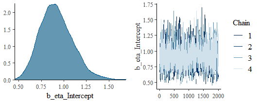
  • What is the posterior distribution of Intercept in the intercep model?
  • Could you share a (subset of) the data you are working with to let me try this locally?

I’ll also note that brms does by default center (but not scale) predictors when an intercept is present and the prior is on the intercept for this centered model (estimate is then reported for the intercept as if centering did not happen, the centering does not affect estimates of other parameters in any way). So that might also cause some discrepancy.

Best of luck with your model!

1 Like

No need to apologize: I know this forum gets busy, and I just appreciate any help figuring this problem out.

Here are the posteriors of the intercept term on the easiness (eta) and discrimination (logalpha) parameters (just taken from plot(TwoPL_inter, "b_eta_Intercept")):

image

image

As far as providing the data, I unfortunately can’t share the actual data, but I did fit the data in the mirt package using run-of-the-mill IRT and then used those results to simulate data: SimulatedData.csv (874.6 KB)

1 Like

I admit I am still not completely sure what is happening, but there are a few pointers.

There is a bit of a difference in variance of the prior distribution: when you include intercept, the prior("normal(0, 2)", class = "b", nlpar = "eta") translates to N(0,2) prior for Item1 but N(0, sqrt(2) * 2) prior for other items (because those are represented as the sum of N(0,2) - distributed intercept and N(0,2) - distributed effect. When you don’t include intercept, the prior is N(0,2) for all items.

Also I was wrong previously and brms does not seem to center predictors in non-linear models.

The weird part is that when despite the pp_check giving wildly different results, when I look for prior consequences for a specific item and ID, I get very similar results:

NoInt_parameters <- posterior_samples(TwoPL_noint)
Inter_parameters <- posterior_samples(TwoPL_inter)

NoInt_eta <- NoInt_parameters$b_eta_ItemItem_4 + NoInt_parameters$`r_ID__eta[17,Intercept]`
hist(NoInt_eta)

Inter_eta <- Inter_parameters$b_eta_Intercept + Inter_parameters$b_eta_ItemItem_4  + Inter_parameters$`r_ID__eta[17,Intercept]`
hist(Inter_eta)


NoInt_logalpha <- NoInt_parameters$b_logalpha_ItemItem_4
hist(NoInt_logalpha)
Inter_logalpha <- Inter_parameters$b_logalpha_Intercept + Inter_parameters$b_logalpha_ItemItem_4
hist(Inter_logalpha)

NoInt_linpred <- exp(NoInt_logalpha) * NoInt_eta
hist(plogis( NoInt_linpred))
Inter_linpred <- exp(Inter_logalpha) * Inter_eta
hist(plogis(Inter_linpred))

So my only remaining explanation is that the little over-excess of extreme values actually adds up over all items and IDs widening the CI for the overall mean…

But I am quite unsure about this, but don’t have time to investigate deeper at the moment.

Hope that helps at least a little.

This is helpful! For one, it’s reassuring to me that I’m not missing something embarrassingly obvious about the problem, which is good news for someone still learning Stan and Bayesian analyses.

Your insight about the differences in prior effects with and without an intercept is very handy. It’s curious to me that the smaller priors on the items when the intercept is including seemingly improves the model’s performance.

Seems like I do think I need to get the no-intercept model running correctly – just curious to me that it causes such problems for Stan, especially once I start trying other types of models. I wonder whether the fact that some multidimensional models fail to converge reflects the fact that those models are just outright wrong.

I appreciate your help a lot. Any recommendations for others to tag for this kind of problem?

There could be a lot of stuff going on - my current best advice is at Divergent transitions - a primer. I would definitely try running the no-intercept model with wider priors (at least by factor of sqrt(2)). It might also be useful to use different coding of the factor variable (e.g. as outlined at Contrast coding with brms).