I am using cmdstanR to estimate a somewhat complicated model, and am trying to do a visual posterior probability check. I know this is a very simple/basic question, but I can’t seem to find the solution. I can generate the predicted values easily in stan - but I can’t figure out how to easily match the predictions with the covariates used to generate them. There must be an a easy way.
I have a much simpler example using a regression model. Here is the data generation process:
library(simstudy)
library(ggplot2)
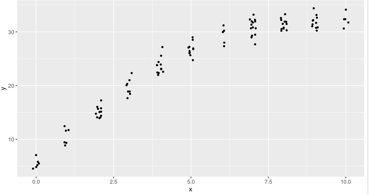
d1 <- defData(varname = "x", formula = "0;10", dist="uniformInt")
d1 <- defData(d1, varname = "y", formula = "5 + 6*x - .3*x^2", variance = 2, dist = "normal")
set.seed(1)
dd <- genData(101, d1)
ggplot(data = dd, aes(x=x, y=y)) +
geom_jitter(height = 0, width = .1, size = 1)
Here is the Stan code:
data {
  int<lower=0> N;
  vector[N] x;
  vector[N] y;
}

parameters {
  real alpha;
  real beta;
  real<lower=0> sigma;
}


model {
  y ~ normal(alpha + beta*x, sigma);
}

generated quantities {
  real y_rep[N] = normal_rng(alpha + beta*x, sigma);
}
And here is the R cmdstanR code:
mod <- cmdstan_model("simple_regression.stan")

fit <- mod$sample(
  data = list(N = nrow(dd), x = dd$x, y = dd$y),
  refresh = 0,
  chains = 2L,
  parallel_chains = 2L,
  iter_warmup = 500,
  iter_sampling = 2500
)

fit$summary()
posterior <- as_draws_array(fit$draws())
The question is - is there an obvious way to attach the predicted values y_rep[1], y_rep[2], etc, with each of the observed values for i=1, 2, …? I am sure I can write code to do this, but if there is a function that will facilitate this, that would be great. I’d like to generate an interval to overlay the observed data. (Clearly, in this case, my model should not be a great fit.)