AR(1) in the error matrix rather than in the linear model

  • Operating System: MacOS
  • brms Version: 2.15.0

This question is related to the recent thread, Unstructured error covariance matrix in a multilevel growth model.

The brms::ar() function appears to set up autoregressive models following the basic format:

y_t \sim \operatorname{Normal}(\alpha + \beta y_{t - 1}, \sigma),

where t indexes time and the autoregressive element is achieved through adding a predictor to the linear model. Is is currently possible to account for autoregression by adding structured correlations to the error matrix rather than adding predictors?

Use case

As in the previous thread, my use case comes from Singer and Willet (2003, Ch 7). This time, I’m looking to fit the model

\begin{align*} \text{opp}_{ij} & \sim \operatorname{Normal}(\mu_{ij}, \mathbf r) \\ \mu_{ij} & = \gamma_{00} + \gamma_{10} \text{time}_{ij} + \gamma_{01} (\text{cog}_i - \overline{\text{cog}}) + \gamma_{11} (\text{cog}_i - \overline{\text{cog}}) \times \text{time}_{ij} \\ \mathbf r & = \begin{bmatrix} \mathbf{\Sigma_r} & \mathbf 0 & \mathbf 0 & \dots & \mathbf 0 \\ \mathbf 0 & \mathbf{\Sigma_r} & \mathbf 0 & \dots & \mathbf 0 \\ \mathbf 0 & \mathbf 0 & \mathbf{\Sigma_r} & \dots & \mathbf 0 \\ \vdots & \vdots & \vdots & \ddots & \mathbf 0 \\ \mathbf 0 & \mathbf 0 & \mathbf 0 & \mathbf 0 & \mathbf{\Sigma_r} \end{bmatrix}, \text{where} \\ \mathbf{\Sigma_r} & = \begin{bmatrix} \sigma^2 & \sigma^2 \rho & \sigma^2 \rho^2 & \sigma^2 \rho^3 \\ \sigma^2 \rho & \sigma^2 & \sigma^2 \rho & \sigma^2 \rho^2 \\ \sigma^2 \rho^2 & \sigma^2 \rho & \sigma^2 & \sigma^2 \rho \\ \sigma^2 \rho^3 & \sigma^2 \rho^2 & \sigma^2 \rho & \sigma^2 \end{bmatrix}. \end{align*}

Is this currently possible with either brms::ar() or some other stragety?

Have you tried ar(cov = TRUE)?

Hey @paul.buerkner, I have. Here’s a focused summary of the results:

The values for Singer and Willett are their point estimates. Those for the two variants fit with brms are the posterior medians. I’m not going to pretend I fully understand what brms is doing, here, but these methods are clearly eating into the residual variance in a way that the REML method is not.

which package are you using for reml?

I’m reporting the REML values straight from the text. However, the IDRE folks fit the models using nlme at Applied Longitudinal Data Analysis, Chapter 7 | R Textbook Examples. Here’s what their model code looked like.

auto1 <- gls(data = opposites,
             opp ~ time*ccog,
             correlation = corAR1(, form = ~ 1 | id), 
             method = "REML")

nlme uses a slightly different paramerization which leads to sigma being no longer sigma but something like sigma / sqrt(1 - ar^2) or something like that (hence higher sigma being reported for higher ar). I am at my phone so please don’t take my word for the formula.

brms parametizes correctly so that sigma is in fact what we expect it to be in this case.

Could you share the link where you’re getting that formula from?

I Googled and found that note in some forum 1 or 2 years or so ago.

you can also verify via simulations of a big enough dataset to see how the implementation differ and verify the correctness of my formula on that basis as well.

Before I dive into a simulation study, it might be helpful if we backed up and clarified a point. When one uses ar(cov = TRUE), is brms fitting an autoregressive model where an autoregressive regression term is added to the linear model, such as in the original formula

y_t \sim \operatorname{Normal}(\alpha + \beta y_{t - 1}, \sigma),

where I’d expect to see a decrease in the residual standard deviation, or is it adding a correlation parameter to the sigma matrix, such as in my use case,

\begin{align*} \text{opp}_{ij} & \sim \operatorname{Normal}(\mu_{ij}, \mathbf r) \\ \mu_{ij} & = \gamma_{00} + \gamma_{10} \text{time}_{ij} + \gamma_{01} (\text{cog}_i - \overline{\text{cog}}) + \gamma_{11} (\text{cog}_i - \overline{\text{cog}}) \times \text{time}_{ij} \\ \mathbf r & = \begin{bmatrix} \mathbf{\Sigma_r} & \mathbf 0 & \mathbf 0 & \dots & \mathbf 0 \\ \mathbf 0 & \mathbf{\Sigma_r} & \mathbf 0 & \dots & \mathbf 0 \\ \mathbf 0 & \mathbf 0 & \mathbf{\Sigma_r} & \dots & \mathbf 0 \\ \vdots & \vdots & \vdots & \ddots & \mathbf 0 \\ \mathbf 0 & \mathbf 0 & \mathbf 0 & \mathbf 0 & \mathbf{\Sigma_r} \end{bmatrix}\\ \mathbf{\Sigma_r} & = \begin{bmatrix} \sigma^2 & \sigma^2 \rho & \sigma^2 \rho^2 & \sigma^2 \rho^3 \\ \sigma^2 \rho & \sigma^2 & \sigma^2 \rho & \sigma^2 \rho^2 \\ \sigma^2 \rho^2 & \sigma^2 \rho & \sigma^2 & \sigma^2 \rho \\ \sigma^2 \rho^3 & \sigma^2 \rho^2 & \sigma^2 \rho & \sigma^2 \end{bmatrix}, \end{align*}

where I wouldn’t expect a decrease in the residual standard deviation because I haven’t added an autoregressive regression term?

it adds a correlation parameter to the sigma matrix. please check the Stan code to verify if you like.

Thank you for the response. I’ve checked the Stan code, but my abilities to read it are quite limited.

It still seems like we’re talking past each other a bit, so let’s simplify the model and the data structure. After making the data, I’ll try to illustrate my basic concern with two simple model. Then I’ll extend the point to variants using ar() and REML.

Data.

Here we make standard bivariate normal data,

\begin{bmatrix} y1 \\ y2 \end{bmatrix} \sim \operatorname{Normal} \left ( \begin{bmatrix} 0 \\ 0 \end{bmatrix}, \begin{bmatrix} 1 & .75 \\ .75 & 1 \end{bmatrix} \right ),

for which N = 10{,}000. We’ll save the data in both the wide (d_wide) and long (d_long) formats.

# load
library(tidyverse)
library(brms)
library(nlme)

# total sample
n <- 1e4

# poplation correlation
rho <- 0.75

# the variance/covariance matrix
Sigma <- 
  matrix(c(1, rho, rho, 1),
         nrow = 2, byrow = T)

# make a wide data set where you might think of
# y1 and y2 as y values at two time points
set.seed(1)

d_wide <- 
  mvtnorm::rmvnorm(n = n, sigma = Sigma) %>% 
  data.frame() %>% 
  set_names(c("y1", "y2")) %>% 
  mutate(id = 1:n())

# make a long version of the data with a single criterion called y,
# which is measured at time == 0 and time == 1
d_long <-
  d_wide %>% 
  pivot_longer(-id, values_to = "y") %>% 
  mutate(time = ifelse(name == "y1", 0, 1))

The data have the sample statistics one would expect.

d_wide %>% 
  summarise(mean1 = mean(y1),
            mean2 = mean(y2),
            sd1 = sd(y1),
            sd2 = sd(y2),
            p = cor(y1, y2))
        mean1        mean2     sd1       sd2         p
1 -0.01297871 -0.001211921 1.00779 0.9971651 0.7511297

Simple models.

We’ll start by fitting two simple models. fit1 is a bivariate normal model with no predictors. Thus the \Sigma matrix is reproduced in the parameters. fit2 is captures the correlation by letting y1 predict y2. However, \sigma_2 is now a residual correlation, and thus quite a bit lower (0.66) than it was in fit1.

# bivariate
fit1 <-
  brm(data = d_wide,
      bf(y1 ~ 1) + bf(y2 ~ 1) + set_rescor(rescor = TRUE))

# pre predicting post
fit2 <-
  brm(data = d_wide,
      y2 ~ 1 + y1)

This exercize is meant to convey my understanding that when a correlation is expressed within the \Sigma matrix (fit1), I would not expect it to eat into the residual variance the way it would when it is expressed, instead, within the linear model (fit2).

Now we get more to the point.

ar().

Instead of fitting AR(1) models with homogeneous variances, as before, I’m going to switch to heterogeneous variances, which will help showcase the issue.

fit3 <-
  brm(data = d_long,
      bf(y ~ time + ar(gr = id),
         sigma ~ 0 + factor(time)))

This does a great job capturing \rho.

posterior_summary(fit3)["ar[1]", -2] %>% round(digits = 2)
Estimate     Q2.5    Q97.5 
    0.74     0.73     0.76 

But look at what happens with the \sigma parameters.

fixef(fit3)[3:4, -2] %>% exp() %>% round(digits = 2)
                  Estimate Q2.5 Q97.5
sigma_factortime0     1.01 0.99  1.02
sigma_factortime1     0.66 0.65  0.67

Whereas the first is a standard deviation, the second is a residual standard deviation.

ar(cov = TRUE).

Now we explore the results when we set cov = TRUE within the ar() function.

fit4 <-
  brm(data = d_long,
      bf(y ~ time + ar(gr = id, cov = TRUE),
         sigma ~ 0 + factor(time)))

As with the previous model, this one does a great job capturing \rho. For the sake of space, I’ll omit the parameter summary. Of greater interest is what happens to the \sigma parameters.

fixef(fit4)[3:4, -2] %>% exp() %>% round(digits = 2)
                  Estimate Q2.5 Q97.5
sigma_factortime0     0.67 0.66  0.67
sigma_factortime1     0.66 0.65  0.67

Now they both appear to be in a residual variance metric. Keeping this in mind, consider what happens when we switch to nlme.

nlme with corAR1() and varIdent().

If you look back at the workflow on the IDRE site, Applied Longitudinal Data Analysis, Chapter 7 | R Textbook Examples, you’ll see one can use nlme to fit an AR(1) model with heterogeneous variances using a combination of the corAR1() and varIdent() functions. Here’s an adaptation of their code applied to our simulated data.

fit5 <- gls(data = d_long,
             y ~ time,
             correlation = corAR1(, form = ~ 1 | id), 
             weights = varIdent(form = ~1 | time),
             method = "REML")

Inspect the results.

print(fit5)
Generalized least squares fit by REML
  Model: y ~ time 
  Data: d_long 
  Log-restricted-likelihood: -24281.95

Coefficients:
(Intercept)        time 
-0.01297871  0.01176678 

Correlation Structure: AR(1)
 Formula: ~1 | id 
 Parameter estimate(s):
      Phi 
0.7511297 
Variance function:
 Structure: Different standard deviations per stratum
 Formula: ~1 | time 
 Parameter estimates:
       0        1 
1.000000 0.989457 
Degrees of freedom: 20000 total; 19998 residual
Residual standard error: 1.00779 

I can’t speak to the equation the nlme package used to compute those \sigma parameters. But it appears, to me, that these residual variances are what I’d expect when (a) the coefficient for time was near zero and the \rho parameter was not eating into the residual variance. This also seems consistent with the models Singer and Willett were discussing in their text. That is, when I fit the model

\begin{align*} y_{ij} & \sim \operatorname{Normal} (\mu_{ij}, \mathbf r) \\ \mu_{ij} & = \beta_0 + \beta_1 \text{time}_{ij} \\ \mathbf r & = \begin{bmatrix} \mathbf{\Sigma_r} & \mathbf 0 & \dots & \mathbf 0 \\ \mathbf 0 & \mathbf{\Sigma_r} & \dots & \mathbf 0 \\ \vdots & \vdots & \ddots & \mathbf 0 \\ \mathbf 0 & \mathbf 0 & \mathbf 0 & \mathbf{\Sigma_r} \end{bmatrix} \\ \mathbf{\Sigma_r} & = \begin{bmatrix} \sigma_1^2 & \sigma_1 \sigma_2 \rho \\ \sigma_1 \sigma_2 \rho & \sigma_2^2 \end{bmatrix}, \end{align*}

where we already know that \beta_1 = 0 because of how we simulated the data, I would expect the \sigma_1 and \sigma_2 parameters to be very close to 1.

So I suppose this leads me back to my original question: Can one fit this model with brms, whether by using the ar() function or by some other means?

What you want in your model is in fact an unstructured residual correlation matrix, which as discussed in the other post, is something that requires a new unst() correlation structure to work in general…

For your simple example with ntimes = 2, you can use ar(cov = TRUE) and get back to the metric you want by comptung sigma_new = sigma / sqrt(1 - ar^2) (on the level of posterior samples). You see this being discussed in more detail on slide 8 ff. in http://bstt513.class.uic.edu/ACerrorsLS.pdf

Does that resolve your question?

1 Like

Thanks @paul.buerkner. Yes, in the special case of two time point data, the heterogeneous autoregressive and unstructured \mathbf{\Sigma_r} matrices are the same. But this breaks down as soon as you have three time points or larger, which is closer to my original use case. For posterity, I’ll walk that through.

Simulate 3-time point data.

# load
library(tidyverse)
library(brms)
library(patchwork)

# total sample
n <- 5e3

# poplation values
s1 <- 1      # standard deviations
s2 <- 2
s3 <- 3
rho <- 0.75  # correlation

# the AR1 variance/covariance matrix
Sigma <- 
  matrix(c(s1 * s1,         s1 * s2 * rho, s1 * s3 * rho^2,
           s2 * s1 * rho,   s2 * s2,       s2 * s3 * rho,
           s3 * s1 * rho^2, s3 * s2 * rho, s3 * s3),
         nrow = 3, byrow = T)

# simulate and wrangle the results into the long format
set.seed(1)

d_long <-
  mvtnorm::rmvnorm(n = n, sigma = Sigma) %>% 
  data.frame() %>% 
  set_names(c("y1", "y2", "y3")) %>% 
  mutate(id = 1:n()) %>% 
  pivot_longer(-id, values_to = "y") %>% 
  mutate(time = ifelse(name == "y1", 0, 
                       ifelse(name == "y2", 1, 2)))

Fit the AR(1) models with both the homogeneous and heterogeneous variaces using the ar(gr = id, cov = TRUE) syntax.

# AR(1) with homogeneous variances
fit6 <-
  brm(data = d_long,
      y ~ time + ar(gr = id, cov = TRUE))

# AR(1) with heterogeneous variances
fit7 <-
  brm(data = d_long,
      bf(y ~ time + ar(gr = id, cov = TRUE),
         sigma ~ 0 + factor(time)))

Extract the posterior draws and wrangle, using Paul’s formula.

sigma <-
  bind_rows(
    # homogeneous variances
    posterior_samples(fit6) %>% 
      transmute(rho = `ar[1]`,
                `sigma[1]` = sigma / sqrt(1 - `ar[1]`^2),
                `sigma[2]` = sigma / sqrt(1 - `ar[1]`^2),
                `sigma[3]` = sigma / sqrt(1 - `ar[1]`^2)),
    # heterogeneous variances
    posterior_samples(fit7) %>% 
      transmute(rho = `ar[1]`,
                `sigma[1]` = exp(b_sigma_factortime0) / sqrt(1 - `ar[1]`^2),
                `sigma[2]` = exp(b_sigma_factortime1) / sqrt(1 - `ar[1]`^2),
                `sigma[3]` = exp(b_sigma_factortime2) / sqrt(1 - `ar[1]`^2))
  ) %>% 
  transmute(`sigma[1]^2` = `sigma[1]`^2,
            `sigma[2]^2` = `sigma[2]`^2,
            `sigma[3]^2` = `sigma[3]`^2,
            `sigma[2]*sigma[1]*rho`   = `sigma[2]` * `sigma[1]` * rho,
            `sigma[3]*sigma[1]*rho^2` = `sigma[3]` * `sigma[1]` * rho^2,
            `sigma[3]*sigma[2]*rho`   = `sigma[3]` * `sigma[2]` * rho,
            `sigma[1]*sigma[2]*rho`   = `sigma[1]` * `sigma[2]` * rho,
            `sigma[1]*sigma[3]*rho^2` = `sigma[1]` * `sigma[3]` * rho^2,
            `sigma[2]*sigma[3]*rho`   = `sigma[2]` * `sigma[3]` * rho)

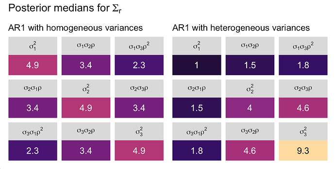
Plot the results.

levels <- c("sigma[1]^2", "sigma[1]*sigma[2]*rho", "sigma[1]*sigma[3]*rho^2",
            "sigma[2]*sigma[1]*rho", "sigma[2]^2", "sigma[2]*sigma[3]*rho",
            "sigma[3]*sigma[1]*rho^2", "sigma[3]*sigma[2]*rho", "sigma[3]^2")

p1 <-
  sigma %>% 
  slice(1:4000) %>% 
  pivot_longer(everything()) %>% 
  group_by(name) %>% 
  summarise(median = median(value)) %>% 
  mutate(cell  = factor(name, levels = levels),
         label = round(median, digits = 1)) %>% 
  
  ggplot(aes(x = 0, y = 0, fill = median, label = label)) +
  geom_tile() +
  geom_text(color = "white") +
  scale_x_continuous(NULL, breaks = NULL, expand = c(0, 0)) +
  scale_y_continuous(NULL, breaks = NULL, expand = c(0, 0)) +
  scale_fill_viridis_c(option = "A", limits = c(0, 10), breaks = NULL) +
  labs(subtitle = "AR1 with homogeneous variances") +
  facet_wrap(~ cell, labeller = label_parsed)

p2 <-
  sigma %>% 
  slice(4001:8000) %>% 
  pivot_longer(everything()) %>% 
  group_by(name) %>% 
  summarise(median = median(value)) %>% 
  mutate(cell  = factor(name, levels = levels),
         label = round(median, digits = 1)) %>% 
  
  ggplot(aes(x = 0, y = 0, fill = median, label = label)) +
  geom_tile() +
  geom_text(aes(color = median < 5)) +
  scale_color_manual(values = c("black", "white"), breaks = NULL) +
  scale_x_continuous(NULL, breaks = NULL, expand = c(0, 0)) +
  scale_y_continuous(NULL, breaks = NULL, expand = c(0, 0)) +
  scale_fill_viridis_c(option = "A", limits = c(0, 10), breaks = NULL) +
  labs(subtitle = "AR1 with heterogeneous variances") +
  facet_wrap(~ cell, labeller = label_parsed)

# combine
p1 + p2 + plot_annotation(title = expression("Posterior medians for "*Sigma[r]))

For comparison, here’s the data-generating variance/covariance matrix.

Sigma %>% round(digits = 1)
     [,1] [,2] [,3]
[1,]  1.0  1.5  1.7
[2,]  1.5  4.0  4.5
[3,]  1.7  4.5  9.0

Conceptually, the brms parameterization still doesn’t make sense, to me. But I’m glad I understand the parameters well enough to transform them into the metric I’m looking for.

indeed please dont use ar() for your 3 time+ use case if your actual target is an unstr matrix. I didn’t mean to imply that. I just used the 2 times procedure to explain to you what the ar() is doing in a case where we have an equivalence.

To clarify, do you mean “please dont use [unst()] for your 3 time+ use case”? The ar() function works great. Also, I almost forgot to say thank you for sharing the link to the slides.

No I just ment that one should not use ar() if what one actually wants is an unstr() matrix for 3+ time points.

That makes sense. Cheers!