Appropriate count distribution for false detection in occupancy models

Hi all,

I am in the process of building an occupancy model that uses data from amplicon sequencing (number of DNA sequences) as its detection model (see Conditional posterior predictions for three-level occupancy model for more details).

To explain the modelling problem, I will first explain briefly the data generating process, and the problem I am encountering. DNA is individually extracted from a set of samples. A marker gene (in my current case, 16S rRNA) is selected for amplification using PCR. The key detail here is that the PCR primers are tagged with a unique forward and reverse index sequence - there are 24 unique forward indices, and 24 unique reverse indexes, for 576 total combinations. Each DNA extract is assigned a unique combination of forward and reverse indices, which allows it to be re-identified later from the sequencing data. Once the samples have been amplified, they are combined together into a single pool of DNA for library preparation and then sequencing. The library is then sequenced, and the resulting sequences are processed through a pipeline that outputs a taxon by sample count matrix.

If this tagging process was perfect, there would be little problem. However, it turns out that during the library preparation, there is a small possibility that these tags to get ‘mixed up’ (called tag jumping or tag switching), which occurs when two molecules that are highly similar or identical, but with different tags, bind together:

image
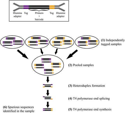
source: https://onlinelibrary.wiley.com/doi/10.1111/1755-0998.13745

This means that there is some level of unknown cross-contamination of samples that occurs during this step, and we can no longer assume that there are no false positives when occupancy modelling.

Luckily, we have data that might allow us to estimate these rates. Not every combination of tags is used, and so this process of tag jumping also recruits sequences into tag combinations that were not used during the PCR stage. In our datasets, we have used approximately 380 tag combinations of the 576, giving roughly 200 unused combinations for which we have data.


There are common ad-hoc methods for dealing with this problem, which typically involve estimating some threshold sequence count and subtracting it from the count matrix (with a floor of zero) - however, this does not seem particularly Bayesian as there will be uncertainty in the number of contaminant seqeunces in each sample.

I have been thinking about how to model this, to account for these false positive detections. Typically when modelling these kind of sequencing counts, a Poisson or Negative binomial is used, with some suitable offset (e.g. total read counts, or geometric means) to account for variation in overall sequencing depth. Here, we can then think of these counts as the sum of two sets of counts - an unknown number of true reads, and an unknown (smaller) number of contaminant reads.

Thinking in the Poisson case for a moment, I think this would allow estimation (for taxon j in sample i) as follows:

Y_{ij} \sim \begin{cases} \textrm{Poisson}(q) & \textrm{for unused combinations} \\ \textrm{Poisson}(p + q) & \textrm{for used combinations} \end{cases}

Where q is the (probably constant) rate of sequence contamination, and p is the true rate of seqence recruitment. This would probably require consideration of some kind of offset for both rates to account for varying sequencing depths.

And extending this to occupancy as follows, for used combinations, with occupancy probability \psi:

Y_{ij} \sim \psi_{ij} \textrm{Poisson}(p + q) + (1 - \psi_{ij})\textrm{Poisson}(q)

The problem is that in reality, the resulting counts are usually overdispersed, and a Poisson fits poorly if at all, so a Negative Binomial with some mean \mu and dispersion \phi is chosen to model these counts. I believe it should be possible to do the same sum of rates as above with a Negative Binomial, but only if the dispersion parameters are equal. However, I don’t think it would be reasonable to expect this is the case - it might even be that the contamination is more closely Poisson distributed, though I haven’t done any empirical poking at this yet.

Can anyone suggest a count distribution, or a method for combining count distributions, that might be appropriate here? I have been thinking about this for a little while, and I am concerned that this could easily be intractable if it requires marginalising over some unknown number of counts (the biggest number of sequences in an unused combination is just over 600).

I don’t have any great mathematical insight here. I will say that if the typical counts are very large, then you can probably get away with approximating them as continuous, and then the problem goes away because the unknown latent parameter giving the number of counts coming from the background is no longer discrete. On the other hand, if the counts are sufficiently small, then it should be tractable to explicitly marginalize over all possibilities for how the sum is achieved. There might possibly be a no man’s land where the marginalized likelihood evaluation is expensive but the continuous approximation is hopelessly poor. Note however that expensive likelihood evaluations are what reduce_sum is great at. I suspect that this no man’s land might not truly exist if you have access to HPC resources.

Note that in N-mixture models the standard way that we evaluate the likelihood is by marginalizing up to some sufficiently large value, so likelihoods with up to hundreds of terms in the marginalization are known to be sufficiently fast in some applications.

Thanks for the thoughts! I’ve been mulling this over in my head the past week and I have had a few more thoughts since.

First, just to reiterate that the main parameter that we are interested in is \psi_{ij}, the probability that a sample i truly contains sequences from species j. Being able to model the number of ‘uncontaminated/true positive’ reads directly is a nice-to-have, but I don’t think it is necessary for inference. Thus, I was thinking it might be possible to build the model as a mixture of two count distributions:

\lambda_{ij} = p_{ij} + q_{ij} \\ Y_{ij} \sim \begin{cases} \textrm{NegBin}(\lambda_{ij}, \phi_{true}) & \textrm{when} Z_{ij} = 1 \\ \textrm{NegBin}(q_{ij}, \phi_{false}) & \textrm{when} Z_{ij} = 0 \\ \end{cases}

And parameterise \lambda_{ij} directly. This wouldn’t model the signature of contaminants vs true sequences directly, but would hopefully allow separating the occupancy rate as we should always expect (p + q) > q.


However, you’ve had me thinking about the possibility of marginalisation, and I don’t think it’s insurmountable. My intuition (thinking about it) is that we only need to marginalise over one count type, as Y_{ij} is the sum of just two types of count. There are two things that I think make this tractable:

  1. Regarding the counts, Y_{ij} can vary in magnitude from single digits to 1000s or even in a few cases 100000s, with most counts being small. However, the number of contaminant reads in the unused combinations is always small - in the dataset I’m looking at currently, the maximum is about 600, though the maximum after filtering unwanted species (I get a lot of mitochondrial reads, another problem!) is only about 150. This will obviously vary by dataset, but I don’t think marginalising over 0:1000 would be terribly hard.
  2. There’s a natural cap on the maximum number of iterations, which is Y_{ij} itself - if there are only 50 reads belonging to species j, there’s no point checking if there’s 51 - 1000 contaminant reads. So for rarer or less abundant species with few read counts we get to make a significant saving. (edit: does this require extra thought - presumably there’s truncation involved here!)

This approach would provide the (nice-to-have) advantage of modelling the true number of reads separately from the contaminant reads. I do indeed have access to HPC resources, so that’s not a problem.

In terms of implementing this, is the idea to iterate over the plausible contamination counts (say, 0:1000), subtract the iteration number from Y_{ij}, get the likelihood of the true counts for each iteration, and take a weighted average according the the probability density of the contaminant counts?

1 Like

This makes a lot of sense if you’re willing to assume that the sum is negative-binomial. But upthread you said that it should be the sum of two negative binomials with different dispersions, which (I think) is not negative binomial. So therein lies the rub :)

Your ideas about marginalization seem spot-on to me.

1 Like

Another way to think about it would be to forget about the sum entirely - assuming presence, reads are drawn from one negative binomial, and assuming absence, another, without the assumption that there is explicit contamination.

That’s reassuring to hear 😁

With regards to the case in point #2 above: say Y_{ij} is 50. The maximum number of contaminant reads this sample could have is thus also 50. However, the distribution implied by say, \textrm{Poisson}(q) or \textrm{Negative Binomial}(q) is unbounded and thus could permit values higher than 50. In this case, where Y_{ij} < N_{iter}, should the likelihoods for each iteration be weighted by the standard distribution for q (say, poisson_lpmf(q), or a truncated version (poisson_lpmf(q)T(0, Y_{ij})), as there is a hard cap on the number of possibilities? I suspect the latter may imply some different distribution that is unwanted!

1 Like

Oooh good question! In this case you don’t need to worry about the truncation, because you aren’t assuming that data-generating-process is truncated. If you thought that 50 was a sample from a sum of truncated negbinomials, then you’d need to worry. But as I understand things, you think that 50 is a sample from a sum of not-truncated negbinomials. So the likelihood for any given breakdown of the sum is the likelihood given the breakdown and the associated (not-truncated) negative binomial parameters.

Note also that even when Y is large (larger than your upper marginalization bound), you can check post-hoc whether your upper marginalization bound was high enough. You want to see that it represents some vanishingly irrelevant upper tail quantile for the fitted negative binomial that gives the distribution of contaminant reads. If you’re right that this distribution has low dispersion and is more nearly Poisson, then this will help you out quite a bit, because with low fitted dispersion the region of irrelevance will begin at much lower values than with high dispersion!

Right. It’s just that if you believe that the underlying process is a sum of two negative binomials with different dispersions, then you implicitly believe that the distribution of reads conditional on presence is not negative binomial. So even if you ignore the fact that it’s a sum and model the count directly, you’re back to the original question, which is what is an appropriate choice of count distribution. Of course, if you’re willing to assume that the distribution of non-contaminant reads is not negative binomial but instead is distributed as the difference between two non-independent negative binomials with different dispersion, then you’re fine. But note that this implies a pretty esoteric, convoluted, and non-simulatable distribution for the true counts. The reason it isn’t simulatable is because to simulate it you would need to first work out the dependency structure between the two binomials (edit: negative binomials), and that seems like a hard problem. (edit: to see intuitively that some dependency structure is required, note that assuming the negative binomials are independent will sometimes result in estimates of negative non-contaminant counts).

1 Like

That’s interesting, I’ll bear that in mind! Unfortunately upon further inspection I’ve found the counts for contamination are far from Poisson - here’s a graph for one of my datasets, where the red ribbon is the 95% PPD for a Poisson regression. X axis is the log10 relative abundance of the species in the whole dataset.

I’ve been struggling to find a good parameterisation for the dispersion in a negative binomial - I’ve been getting credible intervals that are far too high, I think because the outliers throw it off quite a lot. I don’t want to incorporate taxon specific effects though because (fun fact) there are 2347 taxa that don’t appear in these tag switch samples and need to be imputed 🙃 Considering some kind of function of the mean but I need to do more research.

That’s a good point - I’ll definitely go forward with the marginalisation approach. The ideal situation would be to not be in this situation to begin with, but we are out of time and money to do more sequencing…

Do you mean credible intervals for the mean and/or dispersion parameter, or credible intervals for predicted new data?

Apologies - the latter. For comparison, this is a quick and dirty negative binomial for the contaminant reads, letting both the mean and dispersion vary by log10(taxon prevalence). Red ribbon again is 95% PPD - for a lot of mid prevalence taxa (10e-5 to 10e-4), the model allows many taxa to have higher counts than observed. Species-level varying effects help a bit but I haven’t spent much time looking at them.

I am not sure mechanistically why there are some taxa which show such high dispersion. My suspicion from a biological perspective is that the tag jumping process might operate as well with closely-related taxa (in terms of their 16S rRNA sequence), so we might see additional tag switching among these sequences compared to taxa which are more generally dissimilar to one another. But really I have no idea.

I tried coding up the marginalised model, but I’m running into issues with multimodality and divergent transitions:

functions {
  real nb_sum_lpmf(int Y, real SF, real p, real q, real phi, real phi_control, int max_iter) {
    int N_iter;
    if(Y < max_iter) {
      N_iter = Y;
    } else {
      N_iter = max_iter;
    }
    
    vector[N_iter + 1] weighted_probs;
    for(i in 0:N_iter){
      weighted_probs[i + 1] = neg_binomial_2_log_lpmf(i | q, phi_control) + 
        neg_binomial_2_log_lpmf(Y - i | log(SF) + p, phi);
    }
    
    return log_sum_exp(weighted_probs);
  }
}
data {
  int N_samples;                    // Number of samples
  int N_controls;                   // Number of controls
  array[N_samples] int Y;           // Raw data 
  vector[N_samples] SF;             // Size factors
  array[N_controls] int Y_control;  // Raw data (controls)

  // Site occupancy predictors
  int N_pred_occ;                      // Number of occupancy predictors
  matrix[N_samples, N_pred_occ] X_occ; // Predictor matrix for occupancy
  
  // Read abundance predictors
  int N_pred_reads;                        // Number of read predictors
  matrix[N_samples, N_pred_reads] X_reads; // Predictor matrix for reads
}
parameters {
  // Site occupancy parameters
  vector[N_pred_occ] b_occ;

  // Read abundance parameters
  vector[N_pred_reads] b_reads;
  real<lower=0> phi;

  // Contamination parameters
  real q;
  real<lower=0> phi_contam;
}
model {
  // Priors
  // Occupancy
  target += normal_lpdf(b_occ | 0, 10);

  // Read abundance 
  target += normal_lpdf(b_reads | 0, 10);
  target += exponential_lpdf(phi | 1);

  // Contamination
  target += normal_lpdf(q | 0, 10);
  target += exponential_lpdf(phi_contam | 1);

  vector[N_samples] p = X_reads * b_reads;
  vector[N_samples] psi = X_occ * b_occ;
  
  // Likelihood
  for(i in 1:N_samples){
    target += log_sum_exp(
      bernoulli_logit_lpmf(1 | psi) + nb_sum_lpmf(Y[i] | SF[i], p[i], q, phi, phi_contam, 1000),
      bernoulli_logit_lpmf(0 | psi) + neg_binomial_2_log_lpmf(Y[i] | q, phi_contam)
    );
  }
  
  for(i in 1:N_controls) {
    target += neg_binomial_2_log_lpmf(Y[i] | q, phi_contam);
  }
}

Simulate data

library(tidyverse)
library(cmdstanr)

sim_fd_data <- function(
  N_samples = 150,
  N_controls = 50,
  b_occ,
  a_contam,
  b_reads,
  phi,
  phi_contam
) {
  
  ## Generate simulated data
  X_samples <- tibble(
    Intercept = rep(1, N_samples),
    V1 = rnorm(N_samples, 0, 3)
  ) |> 
    mutate(logit_psi = b_occ[1] * Intercept + b_occ[2] * V1,
           psi = plogis(logit_psi),
           Z = rbinom(1, 1, psi),
           q_reads = rnbinom(N_samples, mu = a_contam, size = phi_contam),
           log_p = b_reads[1] * Intercept + b_reads[2] * V1,
           SF = rgamma(N_samples, 5, 2),
           p = exp(log_p),
           p_reads = rnbinom(N_samples, mu = log(SF) + p, size = phi),
           reads = q_reads + p_reads)
    
  X_contam <- tibble(
    reads = rnbinom(N_controls, mu = a_contam, size = phi_contam)
  )
  
  stan_data <- list(
    N_samples = N_samples,
    N_controls = N_controls,
    Y = X_samples$reads,
    SF = X_samples $SF,
    Y_control = X_contam$reads,
    N_pred_occ = 2,
    X_occ = select(X_samples, Intercept, V1) |> as.matrix(),
    N_pred_reads = 2,
    X_reads = select(X_samples, Intercept, V1) |> as.matrix()
  )
  
  return(list(
    true_X_samples = X_samples,
    true_X_contam = X_contam,
    stan_data = stan_data
  ))
}

sim <- sim_fd_data(
  N_samples = 150, 
  N_controls = 50, 
  b_occ = c(0, 3), 
  a_contam = 20, 
  b_reads = c(3, 1), 
  phi = 5, 
  phi_contam = 0.5
  )

model <- cmdstan_model("stan/sgcp_fd_nb_1spp.stan")
fit <- model$sample(data = sim$stan_data, chains = 4, parallel_chains = 4)

The above returns about 100 divergent transitions, and the posterior summary is quite funky, with high Rhats and low ESS. The estimates all look pretty much completely wrong, except for maybe phi_contam (although it’s multimodal). I’ve looked over the implementation and I think I’ve caught all the obvious things (implementation problems, parameters on wrong scale or untransformed, etc.).

   variable     mean   median     sd    mad       q5      q95 rhat ess_bulk ess_tail
 lp__       -1223.93 -1227.39 111.83 166.13 -1338.47 -1110.04 1.74        6      185
 b_occ[1]       0.00    -0.28  18.79  25.61   -25.22    25.13 1.73        6      229
 b_occ[2]      -0.03    -0.04   1.04   1.00    -1.69     1.69 1.03      412     1019
 b_reads[1]     1.08     2.16   7.23   0.52   -13.12    12.66 1.67     1708      357
 b_reads[2]     0.31     0.96   7.17   0.18   -13.30    12.12 1.72     2502      148
 phi            2.08     2.37   1.36   1.67     0.11     4.06 1.46        7      250
 q              5.48     5.42   1.46   2.14     3.88     7.14 1.74        6      151
 phi_contam     0.35     0.30   0.12   0.13     0.21     0.54 1.74        6      110

One element I’m not so sure about is the likelihood for the controls - if I was writing an occupancy model, for samples with confirmed detections one would write log(psi) + dist(Y | params), which by analogy here would be log(1 - psi) + neg_binomial(Y | q, phi_control). But in this case, the controls are not samples - they are a-priori unoccupied, and even if they weren’t, it’s not clear what value of psi they would need to take, given that it is defined as a function of sample properties, not control properties. Is that correct, or does this likelihood also need the additional term?


edit: I tried coding up a simpler version of the above using two Poisson distributions, as for these there is an analytic solution (poisson_lpmf(p + q)). While this version doesn’t give divergences, it also shows severe bimodality, worse even than in the model above. So it seems that it might be a more fundamental problem with the approach above, than to do with my implementation of the marginalisation.

In case anyone else comes across this looking for a solution: after some more soul searching and bug fixing, I have a working solution. What I was missing from my code above (apart from the many bugs I missed) was that the contaminant element of the problem is not actually part of the occupancy problem, and it doesn’t make sense to think of these ‘unused’ combinations as samples - instead they are measures of the additional noise in the reads. Thus, we need to marginalise across the whole occupancy likelihood rather than just the part for Z = 1, which also allows us to factor the occupancy marginalisation within the loop properly to account for when Y is zero or not.

functions {
  real pois_occ_diff_lpmf(int Y, real psi, real p, real q, int max_iter) {
    int N_iter;
    if(Y < max_iter) {
      N_iter = Y;
    } else {
      N_iter = max_iter;
    }
    
    vector[N_iter + 1] weighted_probs;
    for(i in 0:N_iter){
      int Y_iter = Y - i;
      
      if(Y_iter > 0) {
        weighted_probs[i + 1] = bernoulli_logit_lpmf(1 | psi) + poisson_log_lpmf(Y_iter | p);
      } else {
        weighted_probs[i + 1] = log_sum_exp(
          bernoulli_logit_lpmf(1 | psi) + poisson_log_lpmf(Y_iter | p),
          bernoulli_logit_lpmf(0 | psi)
        );
      }
      
      weighted_probs[i + 1] += poisson_log_lpmf(i | q);
      
    }
    
    return log_sum_exp(weighted_probs);
  }
}
data {
  int N_samples;                    // Number of samples
  int N_controls;                   // Number of controls
  array[N_samples] int Y;           // Raw data 
  vector[N_samples] SF;             // Size factors
  array[N_controls] int Y_control;  // Raw data (controls)

  // Site occupancy predictors
  int N_pred_occ;                      // Number of occupancy predictors
  matrix[N_samples, N_pred_occ] X_occ; // Predictor matrix for occupancy
  
  // Read abundance predictors
  int N_pred_reads;                        // Number of read predictors
  matrix[N_samples, N_pred_reads] X_reads; // Predictor matrix for reads
}
parameters {
  // Site occupancy parameters
  vector[N_pred_occ] b_occ;

  // Read abundance parameters
  vector[N_pred_reads] b_reads;

  // Contamination parameters
  real q;
}
model {
  // Priors
  // Occupancy
  target += normal_lpdf(b_occ | 0, 3);

  // Read abundance 
  target += normal_lpdf(b_reads | 0, 3);

  // Contamination
  target += normal_lpdf(q | 0, 3);

  // Calculate predictors
  vector[N_samples] p = (X_reads * b_reads) + SF;
  vector[N_samples] psi = X_occ * b_occ;
  
  // Likelihood
  for(i in 1:N_samples){
    target += pois_occ_diff_lpmf(Y[i] | psi[i], p[i], q, 1000);
  }
  
  for(i in 1:N_controls) {
    target += poisson_log_lpmf(Y_control[i] | q);
  }
}

sim_fd_pois_data <- function(
  N_samples = 150,
  N_controls = 50,
  psi,
  a_contam,
  a_det
) {
  
  ## Generate simulated data
  X_samples <- tibble(Z = rbinom(N_samples, 1, psi),
                      SF = rgamma(N_samples, 5, 2)) |> 
    mutate(reads = rpois(N_samples, lambda = exp((Z * (SF + a_det))) + exp(a_contam)))
    
  X_contam <- tibble(
    reads = rpois(N_controls, lambda = exp(a_contam))
  )
  
  stan_data <- list(
    N_samples = N_samples,
    N_controls = N_controls,
    Y = X_samples$reads,
    SF = X_samples$SF,
    Y_control = X_contam$reads,
    N_pred_occ = 1,
    N_pred_reads = 1,
    X_occ = matrix(rep(1, N_samples)),
    X_reads = matrix(rep(1, N_samples))
  )
  
  return(list(
    true_X_samples = X_samples,
    true_X_contam = X_contam,
    stan_data = stan_data
  ))
}

sim_pois <- sim_fd_pois_data(
  N_samples = 150, 
  N_controls = 50, 
  psi = 0.5,
  a_det = 5,
  a_contam = 2
)

## Marginalised poisson
model_pois_marg <- cmdstan_model("stan/sgcp_fd_pois_marg.stan")
fit_pois_marg <- model_pois_marg$sample(data = sim_pois$stan_data, chains = 4, parallel_chains = 4)
variable  mean median      sd     mad    q5   q95  rhat ess_bulk ess_tail
psi      0.499  0.499 0.0401  0.0409  0.434 0.565  1.00    2533.    2602.
a_det    5.00   5.00  0.00190 0.00193 5.00  5.01   1.00    4712.    2776.
a_contam 2.06   2.06  0.0325  0.0333  2.01  2.12   1.00    2568.    2470.

The only issue I have is that the chains seem to have a lot of trouble getting to where they need to be - some chains take a lot more time than others. In the run above, they took 215.6s, 216.1s, 280.8s, and 288.6s. I am not sure why this is, and whether or not it is a problem - one possiblilty is that certain parameter combinations are just inherently slower in the marginalisation loop above, so some chains might just take longer? The other possibility is that the model has some hard to explore geometry and some chains get stuck - in which case, I am not sure what to do or whether it’s possible to reparameterise. I am concerned that these problems might be more problematic when moving from a simple Poisson intercept model to a complex multi-species model with Negative binomials…

Looking at the trace plots, there’s definitely a little bit of evidence of autocorrelation? Here’s the plot for psi:

1 Like

I’ve been having quite a bit of trouble with the model as specified above, when testing it on my own data - it pretty much unilaterally predicts occupancy as the proportion of samples with reads, regardless of contamination. Upon reflection, I first thought that I was simply predicting poorly the number of contaminants, and improved the model for prediction (there’s a geometric element to this problem due to the combinatorial nature of the issue), but this didn’t work either. However, in working on this I realised that the model above gets the generative model wrong.

Instead of each sample containing some number of contaminant reads, it’s more correct to think of the total read pool for a taxon as some fixed number. When the tag jumping process occurs, sequences switch out of their original sample into another. Samples with zero sequences for a taxon initially can only gain reads, but samples that initially contained reads can both gain and lose them, with rates proportional to the number of reads available to switch between any pair of tag combinations. Thus, the problem only manifests as ‘contamination’ in samples that originally contained no sequences, and elsewise the number of reads could either be larger or smaller.

Considering this, I have implemented a new model: in a standard occupancy model, we assume that any number of detections (Y_{ij} > 0) guarantees a confirmed presence. Instead, we can model the number of reads required for a confirmed presence using a negative binomial model of the reads from unused combinations, and marginalise over all plausible outcomes. This model gives much more sensible results when run on real data, and I think makes intuitive sense - we cannot be confident a taxon is present until it is higher than some threshold number of reads we see as noise in the data.


The question I have now is how to extend this model to two layers of occupancy. In my original (no false detection) model, samples are clustered within sites, and the predictors for occupancy at the site level differ from those at the within site level. The likelihood looks like the following, where Q_{ijk} is 1 if any sample at a site is occupied and 0 otherwise:

[y_{ijk} \mid \psi_{ij}, \theta_{ijk}] = \begin{cases} \psi_{ij} \left( \prod_{k = 1}^{K} \theta_{ijk}[y_{ijk} \mid p_{ijk}, u_{ijk} = 1] + \\(1 - \theta_{ijk})I(R_{ijk} = 0) \right)&\text{if } Q_{ijk} = 1 &\\ \psi_{ij} \left( \prod_{k = 1}^{K} \theta_{ijk}[y_{ijk} \mid p_{ijk}, u_{ijk} = 1] + \\(1 - \theta_{ijk}) \right) + (1 - \psi_{ij}) &\text{if } Q_{ijk} = 0 \end{cases}

However, I’m not quite sure how to work the marginalisation. There seem to be three possibilities:

  1. Marginalise for each sample individually, and then use only the likelihood for Q = 0. I tested this first and it does not fit well.
  2. Marginalise over the whole likelihood, using a single loop over all samples.
  3. Marginalise over the whole likelihood, but each sample is marginalised individually and thus we consider all possible combinations of the threshold across each set of samples.

I think 2 would be workable, if slow, but three obviously would be intractable (some sites have 45 samples). My intuition varies a little depending on the moment, but my suspicion is that 3) is probably correct, given that the samples are independent within sites?