Another option is to use Gelman’s hierarchical ANOVA approach (Gelman, 2005; Analysis of variance—why it is more important than ever). The difficulty with that approach is often times the factor variables have a small number of categories, such as with cyl and gear, both of which only have 3 categories. Thus to help the HMC algorithm along, you might try:
- standardizing the criterion variable
mpg;
- using regularizing priors, particularly for the level-2 \sigma parameters; and/or
- fiddling with the
control settings, such as adapt_delta.
Here’s how that can work with your example.
# load packages
library(tidyverse)
library(brms)
library(tidybayes)

# fit the model
anova1 <- brm(
    # notice we're standardizing the criterion
    data = mtcars %>% mutate(mpgz = (mpg - mean(mpg)) / sd(mpg)),
    family = gaussian,
    # here's the basic formula for the hierarchical ANOVA
    mpgz ~ 1 + (1 | cyl) + (1 | gear) + (1 | carb),
    # here are our regularizing priors
    prior = prior(normal(0, 1), class = Intercept) +
        prior(exponential(1), class = sd) +
        prior(exponential(1), class = sigma),
    cores = 4, seed = 1,
    # notice how this increased the adapt_delta setting
    control = list(adapt_delta = .95)
)
To compare the relative importance of the factor variables, we look at the magnitudes of the level-2 \sigma posteriors. Those appear in the Group-Level Effects section of the summary() output.
summary(anova1)
 Family: gaussian
  Links: mu = identity; sigma = identity
Formula: mpgz ~ 1 + (1 | cyl) + (1 | gear) + (1 | carb)
   Data: mtcars %>% mutate(mpgz = (mpg - mean(mpg))/sd(mpg) (Number of observations: 32)
  Draws: 4 chains, each with iter = 2000; warmup = 1000; thin = 1;
         total post-warmup draws = 4000

Group-Level Effects:
~carb (Number of levels: 6)
              Estimate Est.Error l-95% CI u-95% CI Rhat Bulk_ESS Tail_ESS
sd(Intercept)     0.32      0.28     0.01     1.04 1.00      787     1114

~cyl (Number of levels: 3)
              Estimate Est.Error l-95% CI u-95% CI Rhat Bulk_ESS Tail_ESS
sd(Intercept)     0.90      0.53     0.12     2.24 1.00     1183      837

~gear (Number of levels: 3)
              Estimate Est.Error l-95% CI u-95% CI Rhat Bulk_ESS Tail_ESS
sd(Intercept)     0.43      0.40     0.02     1.48 1.00     1232     2046

Population-Level Effects:
          Estimate Est.Error l-95% CI u-95% CI Rhat Bulk_ESS Tail_ESS
Intercept     0.04      0.54    -1.02     1.13 1.00     1758     2179

Family Specific Parameters:
      Estimate Est.Error l-95% CI u-95% CI Rhat Bulk_ESS Tail_ESS
sigma     0.54      0.08     0.41     0.72 1.00     2536     2254

Draws were sampled using sampling(NUTS). For each parameter, Bulk_ESS
and Tail_ESS are effective sample size measures, and Rhat is the potential
scale reduction factor on split chains (at convergence, Rhat = 1).
This might be easier to see in a plot.
as_draws_df(anova1) %>%
    pivot_longer(starts_with("sd_")) %>%
    mutate(name = str_replace(name, "sd_", "sigma[") %>% str_replace("__Intercept", "]")) %>%

    ggplot(aes(x = value, y = name)) +
    stat_halfeye() +
    scale_y_discrete(NULL, labels = ggplot2:::parse_safe, expand = expansion(mult = 0.05)) +
    xlab("posterior")
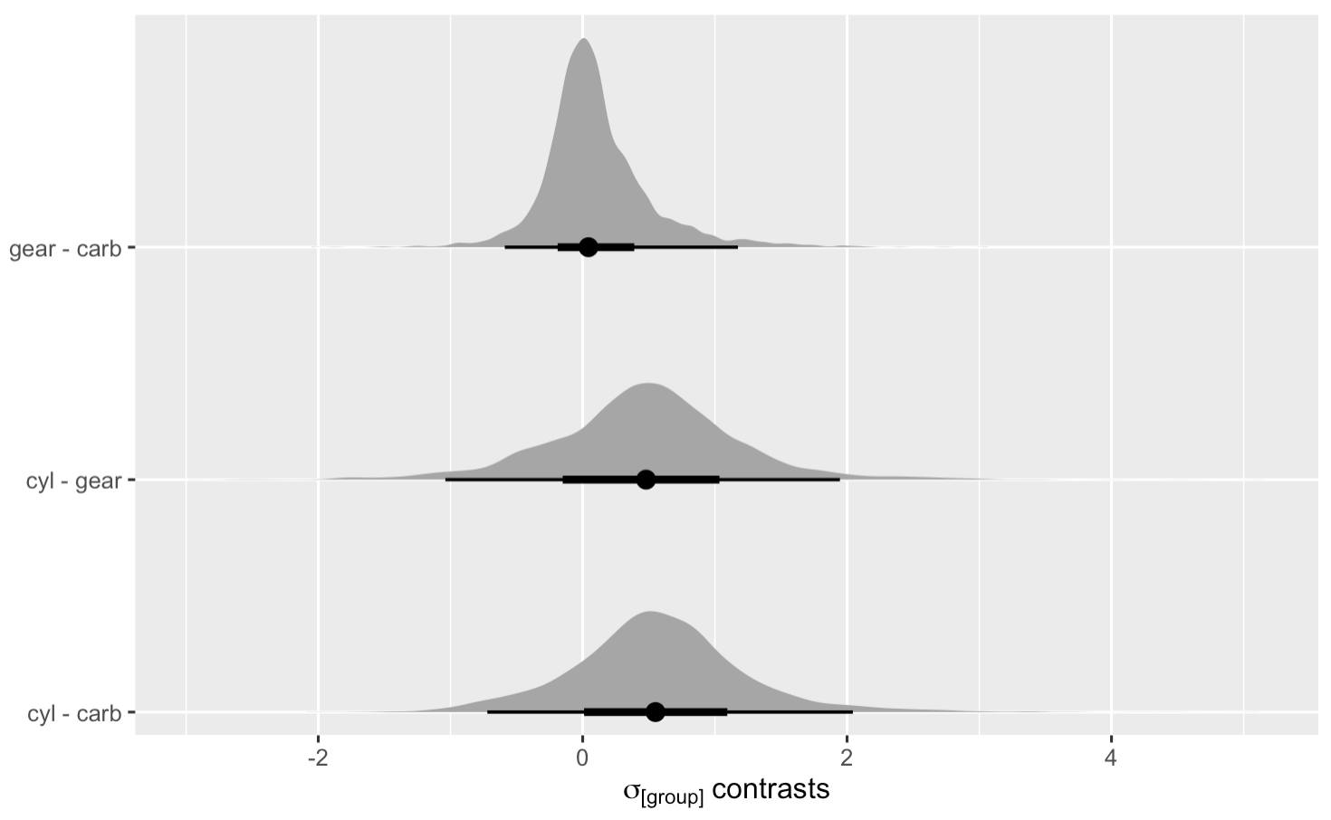
Even with all our tricks, the posteriors for \sigma_\text{carb} and \sigma_\text{gear} look a little rough, but again, that’s what often happens when you fit upper-level \sigma parameters with so few factor levels. But anyways, the cyl factor looks like it’s the most important. We can even formally compare the \sigma posteriors with contrast distributions.
as_draws_df(anova1) %>%
    pivot_longer(starts_with("sd_")) %>%
    mutate(name = str_remove(name, "sd_") %>% str_remove("__Intercept")) %>%
    mutate(name = factor(name, levels = c("carb", "gear", "cyl"))) %>%
    compare_levels(value, by = name, comparison = "pairwise")  %>%

    ggplot(aes(x = value, y = name)) +
    stat_halfeye() +
    scale_y_discrete(NULL, expand = expansion(mult = 0.05))  +
    xlab(expression(sigma["[group]"]~contrasts))
Those contrast distributions reveal the uncertainty in our comparisons. Sure, cyl looks like it’s the best, but with so few levels within each grouping variable, we should remain skeptical.