Thanks. Here’s the Stan code:
transformed data {
  real r = 10;
  real A = 6;
  real omega = 6;
}
parameters {
  vector[2] x;
}
model {
  target += -0.5 * (hypot(x[1], x[2]) + r + A * cos(omega * atan2(x[2], x[1])));
}
This is probably another good case for convergence diagnoistics. Here’s the RStan call:
fit <- sampling(model,
                control = list(stepsize = 0.01, adapt_delta = 0.999, max_treedepth=11),
                chains = 4, iter = 50000)
There was still one iteration that exceed max treedepth 11 and one divergent iteration among the 100K iterations.
     mean se_mean   sd  2.5%   25%   50%   75% 97.5% n_eff Rhat
x[1]  0.15    0.15 3.35 -7.06 -1.32  0.03  1.79  7.22   499 1.01
x[2] -0.09    0.15 3.42 -7.15 -2.10 -0.17  1.95  6.78   518 1.01
lp__ -4.53    0.02 1.60 -8.54 -5.35 -4.20 -3.35 -2.41  7576 1.00
Nevetheless, it looks like the true posterior means (which should be zero) are within standard error, but that n_eff is terrible. This is 100K draws! We start to get nervous when the effective sample size rate is 200 draws. Stan’s definitely not exploring this posterior well, though I get the feeling it’d get there with more draws and ideally more chains.
Because of the low n_eff, the standard error for the means is pretty bad. I’m not sure what the true posterior sd is supposed to be. Although it appears to be roughly symmetric for x[1] and x[2], it may not be getting far enough into the tails.
Here’s the code for the plot:
> post_x <- extract(fit)$x
> post_x1 <- post_x[ , 1]
> post_x2 <- post_x[ , 2]
> df <- data.frame(x1 = post_x1, x2 = post_x2)
> plot(post_x1, post_x2)
> library(ggplot2)
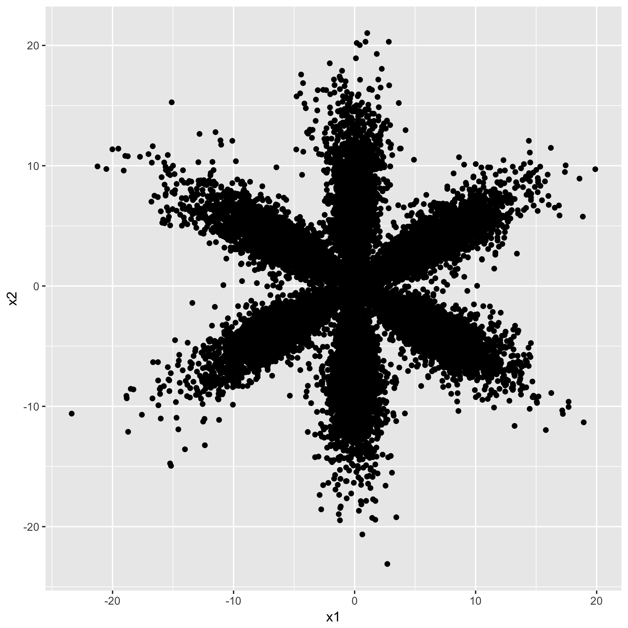
> ggplot(df, aes(x1, x2)) + geom_scatterplot()
Which is why we odn’t evaluate these things by eye:
So I tried 16 chains with some thinning so as not to kill my machine:
fit <- sampling(model, chains=16, iter=50000, thin = 25,
                control=list(adapt_delta=0.999,
                             stepsize=0.999,
                             max_treedepth=11))
It takes about 20s/chain on my Mac notebook (6-year old i7). This produces much better results, as one might expect, with a total of 16K saved posterior draws.
> print(fit)
Inference for Stan model: flower.
16 chains, each with iter=50000; warmup=25000; thin=25;
post-warmup draws per chain=1000, total post-warmup draws=16000.

      mean se_mean   sd  2.5%   25%   50%   75% 97.5% n_eff Rhat
x[1] -0.04    0.07 3.45 -7.37 -1.71 -0.02  1.61  7.35  2322 1.01
x[2] -0.05    0.07 3.44 -7.04 -2.06 -0.19  2.00  6.79  2271 1.01
lp__ -4.56    0.01 1.62 -8.60 -5.39 -4.21 -3.37 -2.44 15039 1.00
The sd are even a little higher. As you can see, 2.5% and 97.5% intervals are terrible. This may be indicating poor tail exploration, but they’re still within MCMC standard error here because 2.5% tail probabiliites only use about 1/40 of the draws, meaning 1/sqrt(40) the effective sample size, which is still decent here at around 300.