ODE non-converging; Rhat beyond 1

[irenegfsr]

Thanks that worked.
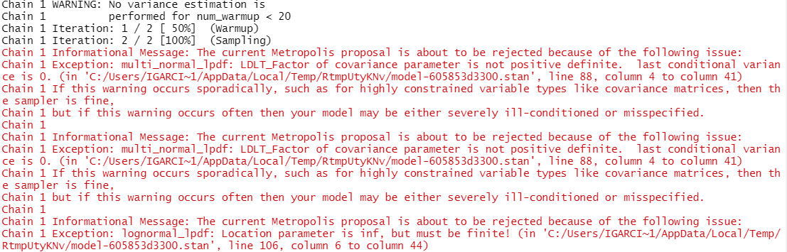
However, I am still struggling with error messages as follows:

So at least the model runs now, but I am facing divergence issues due to the specification of the variance-covariance matrix. However, I have reviewed this and try different covariance matrices but they all gave the same error message.
The code is as follows:

functions {
  real[] analytic_int(real[] inits, real t0, real ts, real[] theta) {
    real y[3];
    real dt = ts - t0;
    real C;
    y[1] = inits[1]*exp(-theta[1]*dt);
    y[2] = inits[2]*exp(-theta[2]*dt);
    C = inits[3] + inits[1]*theta[1]/(theta[1]-theta[3]) + inits[2]*theta[2]/(theta[2]-theta[3]);
    y[3] = theta[1]*y[1]/(theta[3] - theta[1]) + theta[2]*y[2]/(theta[3] - theta[2]) + C*exp(-theta[3]*dt);
    return inits;
  }
}
data {
  int<lower=1> N;
  int<lower=1> nsubjects;
  int<lower=1> subj_ids[N];
  real <lower=0> y[N];
  int <lower=1> ntimes;
  int <lower=1> nobs[nsubjects];
  real ts[ntimes];
  real t0;
}
transformed data {
    real x_r[0];
    int x_i[0]; 
}
parameters {
  real  logps;
  real  logpl;
  real  logmuab;
  real   sigmalogmuab;
  
  real <lower= 0> logAB0;
  real  sigmalogAB0;
  real  logps0;
  real  logpl0;
  real  sigma;
  
  vector[2] r[nsubjects];
  //real rho_rhobit;
}
model{
  real mu[ntimes, 3];
  real inits[3];
  real theta[3];
  real new_mu[ntimes, 3];
  vector[nsubjects] rAB0;
  vector[nsubjects] rmuab;
  real eval_time[1];
  // transformed parameters 
  real ps = exp(logps);
  real pl = exp(logpl);
  real muab = exp(logmuab);
  real sigma_muab = exp(sigmalogmuab);
  real AB0 = exp(logAB0);
  real sigma_AB0 = exp(sigmalogAB0);
  real ps0 = exp(logps0);
  real pl0 = exp(logpl0);
  real sigmap = exp(sigma);
  // defining the correlation 
  vector[2] mean_vec;
  matrix[2,2] Sigma;
  //real rho = (exp(rho_rhobit) - 1)/(exp(rho_rhobit) + 1);
 
  //prior distributions
  logps ~ normal(0, 1);
  logpl ~ normal(0, 1);
  logmuab ~ normal(0, 10);
  sigmalogmuab ~ normal(0, 1);
  logAB0 ~ normal(5, .5);
  sigmalogAB0 ~ normal(0, 1);
  logps0 ~ normal(0, 1);
  logpl0 ~ normal(0, 1);
  sigma ~ normal(0, 1);
  //rho_rhobit ~ uniform(-10, 10);
  
  //cov matrix
  mean_vec[1] = -pow(sigma_AB0, 2.0)/2;
  mean_vec[2] = -pow(sigma_muab, 2.0)/2;
  
  Sigma[1,1] = pow(sigma_AB0, 2.0);
  Sigma[2,2] = pow(sigma_muab, 2.0);
  Sigma[1,2] = 0;
  Sigma[2,1] = 0;
  
  
  for (j in 1:nsubjects) {
    r[j] ~ multi_normal(mean_vec, Sigma);
    rAB0[j] = r[j,1];
    rmuab[j] = r[j,2];
  }
  for (i in 1:N){
    //defining the initial conditions
    inits[3] = AB0*exp(rAB0[subj_ids[i]]);
    inits[1] = inits[3]/ps0;
    inits[2] = inits[3]/pl0;
    //defining the parameters
    theta[1] = ps;
    theta[2] = pl;
    theta[3] = muab*exp(rmuab[subj_ids[i]]);
    // ode solver
      mu[i] = analytic_int(inits, t0, ts[i], theta);
      new_mu[i,1] = mu[i,1];
      new_mu[i,2] = mu[i,2];
      new_mu[i,3] = log(mu[i,3]) - pow(sigma, 2.0)/2;
      y[i] ~ lognormal(new_mu[i, 3], sigma);
    }
}

[nhuurre]

@irenegfsr

I am still struggling with error messages as follows:

That says there’s a problem with the LDLT factor (aka Cholesky decomposition) of the covariance matrix. I’m not sure why it’s failing; typical cause would be either strong correlation (but the current code has zero correlation) or nonpositve variance (the exp(.) could underflow to zero, i guess?).
You may have better luck when building the Cholesky manually (I’ve included correlation rho too):

matrix[2,2] L_Sigma;
L_Sigma[1,1] = sigma_AB0;
L_Sigma[1,2] = 0.0;
L_Sigma[2,1] = rho*sigma_muab;
L_Sigma[2,2] = sqrt(1-rho*rho)*sigma_muab;
...
r[j] ~ multi_normal_cholesky(mean_vec, L_Sigma);

[irenegfsr]

Why precisely that covariance matrix structure? I think it should be symmetric. Do you think if I rather do a transformation of sigma to; sigma = pow(sigmalogab0, 2.0) instead of the exponential would work? I do believe that it could yield to 0 either way.

[nhuurre]

@irenegfsr

Why precisely that covariance matrix structure? I think it should be symmetric.

It’s a Cholesky factor. The corresponding covariance matrix is

\Sigma=L_{\Sigma}L_{\Sigma}^{T}=\left[\begin{array}{cc} \sigma_{AB}^{2} & \rho\sigma_{AB}\sigma_{\mu}\\ \rho\sigma_{AB}\sigma_{\mu} & \sigma_{\mu}^{2} \end{array}\right]

[irenegfsr]

When I try that structure I

still get the same error message for the covariance matrix plus I also get an error when I call the likelihood

[nhuurre]

That error says multi_normal. Use ~ multi_normal_cholesky(..) instead of ~ multi_normal(..).

[irenegfsr]

Thanks, that worked. However, the error on line 106 still occurs when I call the likelihood.

[nhuurre]

So the lognormal is still failing. You said the model initializes successfully. Does it fail for every iteration or only sometimes?

[nhuurre]

Looking for ways to improve the analytic_int function I only now noticed it ends with

    return inits;

but of course it should be

    return y;

But that makes the latest failure even more mysterious. If it’s returning the inits unchanged then mu should be at least within an order of magnitude of sensible value. So what gives?

And now I see that the parameter sigma has no bounds. The errors are likely result of the sampler trying to explore sigma < 0.

parameters {
  ...
  real<lower=0> sigma;
}

Finally, here’s my improved analytic_int looks like

  real[] analytic_int(real[] inits, real t0, real ts, real[] theta) {
    real y[3];
    real dt = ts - t0;
    real C;
    y[1] = inits[1]*exp(-theta[1]*dt);
    y[2] = inits[2]*exp(-theta[2]*dt);
    y[3] = inits[3]*exp(-theta[3]*dt);
    if (theta[1] == theta[3]) {
      y[3] = y[3] + theta[1]*dt*y[1];
    } else {
      y[3] = y[3] + theta[1]*y[1]*expm1(theta[1]*dt-theta[3]*dt)/(theta[3] - theta[1]);
    }
    if (theta[2] == theta[3]) {
      y[3] = y[3] + theta[2]*dt*y[1];
    } else {
      y[3] = y[3] + theta[2]*y[2]*expm1(theta[2]*dt-theta[3]*dt)/(theta[3] - theta[2]);
    }
    return y;
  }

That expm1(.) is just a more accurate version of exp(.)-1 so this should be equivalent to what we had before.

[irenegfsr]

That’s true it should end with y. I will try the new model block; though I removed the lower bound for sigmas in general because I was getting an error of parameters being too constrained. Even if sigma would be close to 0, it should give a value for y that is not nan of inf, I think.
Are the aforementioned conditions necessary if I still specify that theta has different values in the init function?

[irenegfsr]

@nhuurre

real C;

I have noticed that here you still define C, but the formula is not written. We do not need C in this approach.?

[irenegfsr]

The same error appears…

[nhuurre]

I’ve thought more about this. You’ve said that

• the smallest y is 36
• the largest t is 96
• you initialize the model with list(logps = 1, logpl = 1, logmuab = 1, logAB0 = 5)

And these are kind of inconsistent.

Those inits imply initial value y_3^{t=0}=e^5\approx 148.4 and decay rate \theta_1=\theta_2=\theta_3=e^1\approx2.718.

At that rate t=96 would be about y_3^{0}e^{-t\times \theta_3}=e^5e^{-96\times e}\approx 7\times 10^{-255} which is pretty much zero.

It would be more reasonable to initialize with list(logps = -2, logpl = -2, logmuab = -2) or even list(logps = -3, logpl = -3, logmuab = -3).

[irenegfsr]

I think definitely the initial values have something to do as well with the error message. However, with the following initial values and the previous version of the code (not the one presented below), I get the following error message

Initial values:
initebl2 = function(){
list(logps = -3, logpl = -2, logmuab = -2.5,
sigmalogmuab = 0.5, logAB0 = 3, sigmalogAB0 = 0.7,
logps0 = 1, logpl0 = 1, sigma = 0.6, r = r, rho_rhobit = 0.5)
}

I have been thinking that maybe the times that I have defined play a role in this? My generated time was ascending from 1 to 96 (2081 obs), so real numbers. In reality, the times that I have per subject go kind of like this: (subject1 = 0, 50, 90; subject2 = 0, 49, 70…), some of them 1, 2, or 3 observations.
I have created the eval time to specify what to do when times are 0 with the raw variable time of my data, but I still get this error:

functions {
  real[] analytic_int(real[] inits, real t0, real ts, real[] theta) {
    real y[3];
    real dt = ts - t0;
    real C;
    y[1] = inits[1]*exp(-theta[1]*dt);
    y[2] = inits[2]*exp(-theta[2]*dt);
    C = inits[3] + inits[1]*theta[1]/(theta[1]-theta[3]) + inits[2]*theta[2]/(theta[2]-theta[3]);
    y[3] = theta[1]*y[1]/(theta[3] - theta[1]) + theta[2]*y[2]/(theta[3] - theta[2]) + C*exp(-theta[3]*dt);
    return y;
  }
}
data {
  int<lower=1> N;
  int<lower=1> nsubjects;
  int<lower=1> subj_ids[N];
  real <lower=0> y[N];
  int <lower=1> ntimes;
  int <lower=1> nobs[nsubjects];
  real ts[ntimes];
  real t0;
}
transformed data {
    real x_r[0];
    int x_i[0]; 
}
parameters {
  real  logps;
  real  logpl;
  real  logmuab;
  real  sigmalogmuab;
  
  real <lower= 0> logAB0;
  real  sigmalogAB0;
  real  logps0;
  real  logpl0;
  real   sigma;
  
  vector[2] r[nsubjects];
  real rho_rhobit;
}
model{
  real mu[ntimes, 3];
  real inits[3];
  real theta[3];
  real new_mu[ntimes, 3];
  vector[nsubjects] rAB0;
  vector[nsubjects] rmuab;
  real eval_time[1];
  // transformed parameters 
  real ps = exp(logps);
  real pl = exp(logpl);
  real muab = exp(logmuab);
  real sigma_muab = exp(sigmalogmuab);
  real AB0 = exp(logAB0);
  real sigma_AB0 = exp(sigmalogAB0);
  real ps0 = exp(logps0);
  real pl0 = exp(logpl0);
  real sigmap = exp(sigma);
  // defining the correlation 
  vector[2] mean_vec;
  matrix[2,2] Sigma;
  real rho = (exp(rho_rhobit) - 1)/(exp(rho_rhobit) + 1);
 
  //prior distributions
  logps ~ normal(0, 1);
  logpl ~ normal(0, 1);
  logmuab ~ normal(0, 10);
  sigmalogmuab ~ normal(0, 1);
  logAB0 ~ normal(3, .5);
  sigmalogAB0 ~ normal(0, 1);
  logps0 ~ normal(0, 1);
  logpl0 ~ normal(0, 1);
  sigma ~ normal(0, 1);
  //rho_rhobit ~ uniform(-10, 10);
  
  //cov matrix
  mean_vec[1] = -pow(sigma_AB0, 2.0)/2;
  mean_vec[2] = -pow(sigma_muab, 2.0)/2;
  
  Sigma[1,1] = pow(sigma_AB0, 2.0);
  Sigma[2,2] = pow(sigma_muab, 2.0);
  Sigma[1,2] = rho*sigma_AB0*sigma_muab;
  Sigma[2,1] = rho*sigma_AB0*sigma_muab;
  
  
  for (j in 1:nsubjects) {
    r[j] ~ multi_normal_cholesky(mean_vec, Sigma);
    rAB0[j] = r[j,1];
    rmuab[j] = r[j,2];
  }
  for (i in 1:N){
    //defining the initial conditions
    inits[3] = AB0*exp(rAB0[subj_ids[i]]);
    inits[1] = inits[3]/ps0;
    inits[2] = inits[3]/pl0;
    //defining the parameters
    theta[1] = ps;
    theta[2] = pl;
    theta[3] = muab*exp(rmuab[subj_ids[i]]);
    // ode solver
    eval_time[1] = ts[i];
    if (eval_time[1] == 0){
      new_mu[i,1] = inits[1];
      new_mu[i,2] = inits[2];
      new_mu[i,3] = log(inits[3]) - pow(sigmap, 2.0)/2;}
    else{
      mu[i] = analytic_int(inits, t0, ts[i], theta);
      new_mu[i,1] = mu[i,1];
      new_mu[i,2] = mu[i,2];
      new_mu[i,3] = log(mu[i,3]) - pow(sigma, 2.0)/2;}
      y[i] ~ lognormal(new_mu[i, 3], sigmap);
    }
}

[nhuurre]

That last analytic_int() I posted has some sign errors and sometimes outputs negative values which of course cannot be log()ed. And yes, that real C; was redundant.

I got the following model to run and the results seem kind of reasonable, although effective sample size is low.

functions {
  real[] analytic_int(real[] inits, real t0, real ts, real[] theta) {
    real y[3];
    real dt = ts - t0;
    real C;
    y[1] = inits[1]*exp(-theta[1]*dt);
    y[2] = inits[2]*exp(-theta[2]*dt);
    C = inits[3] + inits[1]*theta[1]/(theta[1]-theta[3]) + inits[2]*theta[2]/(theta[2]-theta[3]);
    if (theta[1] == theta[3] && theta[2] == theta[3]) {
      y[3] = theta[1]*dt*y[1] + theta[2]*dt*y[2] + inits[3]*exp(-theta[3]*dt);
    } else {
       y[3] = theta[1]*y[1]/(theta[3] - theta[1]) + theta[2]*y[2]/(theta[3] - theta[2]) + C*exp(-theta[3]*dt);
    } 
    return y;
  }
}
transformed data {
  // simulate fake data
  int<lower=1> nsubjects = 150;
  int N = 4*nsubjects;
  int <lower=1> nobs[nsubjects];
  int subj_ids[N];
  real <lower=0> y[N];
  int <lower=1> ntimes = N;
  real ts[ntimes];
  real t0 = 0.0;

  {
  real inits[3];
  real theta[3];
  vector[nsubjects] rAB0;
  vector[nsubjects] rmuab;
  vector[2] mean_vec;
  matrix[2,2] Sigma;
  real AB0 = exp(5);
  real muab = exp(-2.5);
  real ps0 = exp(-2.5);
  real pl0 = exp(-2.5);
  real ps = exp(-2.5);
  real pl = exp(-2.5);
  real sigma = 0.5;

  int n_idx = 1;
  for (j in 1:nsubjects) {
    nobs[j] = 4;
    subj_ids[n_idx] = j;
    ts[n_idx] = 0;
    subj_ids[n_idx+1] = j;
    ts[n_idx+1] = 25;
    subj_ids[n_idx+2] = j;
    ts[n_idx+2] = 50;
    subj_ids[n_idx+3] = j;
    ts[n_idx+3] = 75;
    n_idx = n_idx + 4;
    rAB0[j] = 0.0;
    rmuab[j] = 0.0;
  }
  for (i in 1:N){
    inits[3] = AB0*exp(rAB0[subj_ids[i]]);
    inits[1] = inits[3]/ps0;
    inits[2] = inits[3]/pl0;
    theta[1] = ps;
    theta[2] = pl;
    theta[3] = muab*exp(rmuab[subj_ids[i]]);
    //print("t = ", ts[i], "; inits = ", inits, "; theta = ", theta);
    real mu[3] = analytic_int(inits, t0, ts[i], theta);
    real new_mu = log(mu[3]) - pow(sigma, 2.0)/2;
    //print("; mu = ", mu[3], "; new_mu = ", new_mu);
    y[i] = lognormal_rng(new_mu, sigma);
    //print("   y = ", y[i]);
  }
  }
}
parameters {
  real  logps;
  real  logpl;
  real  logmuab;
  real   sigmalogmuab;

  real <lower= 0> logAB0;
  real  sigmalogAB0;
  real  logps0;
  real  logpl0;
  real<lower=0>  sigma;

  vector[2] r[nsubjects];
  //real rho_rhobit;
}
model{
  real mu[ntimes, 3];
  real inits[3];
  real theta[3];
  real new_mu[ntimes, 3];
  vector[nsubjects] rAB0;
  vector[nsubjects] rmuab;
  real eval_time[1];
  // transformed parameters 
  real ps = exp(logps);
  real pl = exp(logpl);
  real muab = exp(logmuab);
  real sigma_muab = exp(sigmalogmuab);
  real AB0 = exp(logAB0);
  real sigma_AB0 = exp(sigmalogAB0);
  real ps0 = exp(logps0);
  real pl0 = exp(logpl0);
  real sigmap = exp(sigma);
  // defining the correlation 
  vector[2] mean_vec;
  matrix[2,2] Sigma;
  //real rho = (exp(rho_rhobit) - 1)/(exp(rho_rhobit) + 1);

  //prior distributions
  logps ~ normal(0, 1);
  logpl ~ normal(0, 1);
  logmuab ~ normal(0, 10);
  sigmalogmuab ~ normal(0, 1);
  logAB0 ~ normal(5, .5);
  sigmalogAB0 ~ normal(0, 1);
  logps0 ~ normal(0, 1);
  logpl0 ~ normal(0, 1);
  sigma ~ normal(0, 1);
  //rho_rhobit ~ uniform(-10, 10);

  //cov matrix
  mean_vec[1] = -pow(sigma_AB0, 2.0)/2;
  mean_vec[2] = -pow(sigma_muab, 2.0)/2;
  
  Sigma[1,1] = pow(sigma_AB0, 2.0);
  Sigma[2,2] = pow(sigma_muab, 2.0);
  Sigma[1,2] = 0;
  Sigma[2,1] = 0;

  for (j in 1:nsubjects) {
    r[j] ~ multi_normal(mean_vec, Sigma);
    rAB0[j] = r[j,1];
    rmuab[j] = r[j,2];
  }
  for (i in 1:N){
    //defining the initial conditions
    inits[3] = AB0*exp(rAB0[subj_ids[i]]);
    inits[1] = inits[3]/ps0;
    inits[2] = inits[3]/pl0;
    //defining the parameters
    theta[1] = ps;
    theta[2] = pl;
    theta[3] = muab*exp(rmuab[subj_ids[i]]);
    // ode solver
    //print("t = ", ts[i], "; inits = ", inits, "; theta = ", theta);
      mu[i] = analytic_int(inits, t0, ts[i], theta);
      new_mu[i,1] = mu[i,1];
      new_mu[i,2] = mu[i,2];
      new_mu[i,3] = log(mu[i,3]) - pow(sigma, 2.0)/2;
    //print("y = ", y[i], "; mu = ", mu[i,3], "; new_mu = ", new_mu[i,3]);
    y[i] ~ lognormal(new_mu[i, 3], sigma);
  }
}

[irenegfsr]

@nhuurre

  {
  real inits[3];
  real theta[3];
  vector[nsubjects] rAB0;
  vector[nsubjects] rmuab;
  vector[2] mean_vec;
  matrix[2,2] Sigma;
  real AB0 = exp(5);
  real muab = exp(-2.5);
  real ps0 = exp(-2.5);
  real pl0 = exp(-2.5);
  real ps = exp(-2.5);
  real pl = exp(-2.5);
  real sigma = 0.5;

  int n_idx = 1;
  for (j in 1:nsubjects) {
    nobs[j] = 4;
    subj_ids[n_idx] = j;
    ts[n_idx] = 0;
    subj_ids[n_idx+1] = j;
    ts[n_idx+1] = 25;
    subj_ids[n_idx+2] = j;
    ts[n_idx+2] = 50;
    subj_ids[n_idx+3] = j;
    ts[n_idx+3] = 75;
    n_idx = n_idx + 4;
    rAB0[j] = 0.0;
    rmuab[j] = 0.0;
  }
  for (i in 1:N){
    inits[3] = AB0*exp(rAB0[subj_ids[i]]);
    inits[1] = inits[3]/ps0;
    inits[2] = inits[3]/pl0;
    theta[1] = ps;
    theta[2] = pl;
    theta[3] = muab*exp(rmuab[subj_ids[i]]);
    //print("t = ", ts[i], "; inits = ", inits, "; theta = ", theta);
    real mu[3] = analytic_int(inits, t0, ts[i], theta);
    real new_mu = log(mu[3]) - pow(sigma, 2.0)/2;
    //print("; mu = ", mu[3], "; new_mu = ", new_mu);
    y[i] = lognormal_rng(new_mu, sigma);
    //print("   y = ", y[i]);
  }
  }
}

I am not sure I understand this part. Except the fact that there are actual values instead of calling the parameters from the parameters block, why would we need that?
Could I also ask how your ts vector look like?

[nhuurre]

The transformed data block was just there so to simulate some data to fit because I don’t have the data you’re using. You can replace that with a simple data block. The times ts are assigned in the nsubjects loop right next to subj_ids; for each subject ts[n_idx:n_idx+3] = {0, 25, 50, 75}.

[irenegfsr]

Right, so the ts goes 0, 25, 50, and 75 per participant? So it is repeating itself continuously?
When I have called in cmdstan your code above, (without data = data) in the sample function, cause you are generating data in Stan, I still get the error message in the likelihood line. Did you also specify initial values for this? How come when you run it it goes smoothly?

[nhuurre]

For me there’s still some warnings at the beginning but those disappear after warmup. You could set inits logps=-3,logmuab=-3 etc but that didn’t seem required.

[nhuurre]

Let’s add some print statements where the code fails:

if (is_nan(new_mu[i,3])) {
  print("t = ", ts[i], "; inits = ", inits, "; theta = ", theta);
  print("y = ", y[i], "; mu = ", mu[i,3], "; new_mu = ", new_mu[i,3]);
}

and now it says

t = 0; inits = [inf,inf,inf]; theta = [3.22315,8.87085e-104,3.26671e-07]
y = 121.409; mu = -nan; new_mu = -nan

The lower bound on logAB0 encourages the sampler to try larger values of AB0 and that easily overflows to infinity.
I don’t see warnings if I set initial stepsize = 0.05