Hey! I’m also no brms expert.
However, I think conceptually, you’d want to do something like this:
bf(
    cum_cases ~ logA - exp(-(exp(logk) * (day_norm - exp(logdelay)))),
    logA ~ 1 + (1 | ID | Country.Region),
    logk ~ 1 + (1 | ID | Country.Region),
    logdelay ~ 1 + (1 | ID | Country.Region),
    nl = TRUE
  )
In the model above there are 2 problems, I think:
- You’ve put a lognormal prior on the common mean of
A, k, and delay. This ensures that the common mean is positive, however, the parameters could still be negative due to the random effect structure. To ensure positivity on the varying parameters, I think you have to wrap them in exp and define everything on the log scale.
- The lognormal “identity” link is essentially a log-link. So i think you do have to take the log of the mean formula if you’re using
family = lognormal().
case_counts$Country.Region <- as.factor(case_counts$Country.Region)
case_counts$day_norm <- case_counts$day/max(case_counts$day)
form_mult2 <-
bf(
cum_cases ~ logA - exp(-(exp(logk) * (day_norm - exp(logdelay)))),
logA ~ 1 + (1 | ID | Country.Region),
logk ~ 1 + (1 | ID | Country.Region),
logdelay ~ 1 + (1 | ID | Country.Region),
nl = TRUE
)
mult_priors2 <- c(
prior(normal(0, 1), nlpar = "logA", lb = 0),
prior(normal(0, 0.5), nlpar = "logk", lb = 0),
prior(normal(0, 0.5), nlpar = "logdelay", lb = 0),
prior(normal(0, 1), class = "sigma"),
prior(
normal(0, 2.5),
class = "sd",
group = "Country.Region",
nlpar = "logA"
),
prior(
normal(0, 1),
class = "sd",
group = "Country.Region",
nlpar = "logk"
),
prior(
normal(0, 1),
class = "sd",
group = "Country.Region",
nlpar = "logdelay"
)
)
modmult2 <- brm(
form_mult2,
data = case_counts,
prior = mult_priors2,
seed = 1234,
family = lognormal(),
chains = 4,
cores = 4,
sample_prior = "no",
control = list(adapt_delta = 0.95, max_treedepth = 15)
)
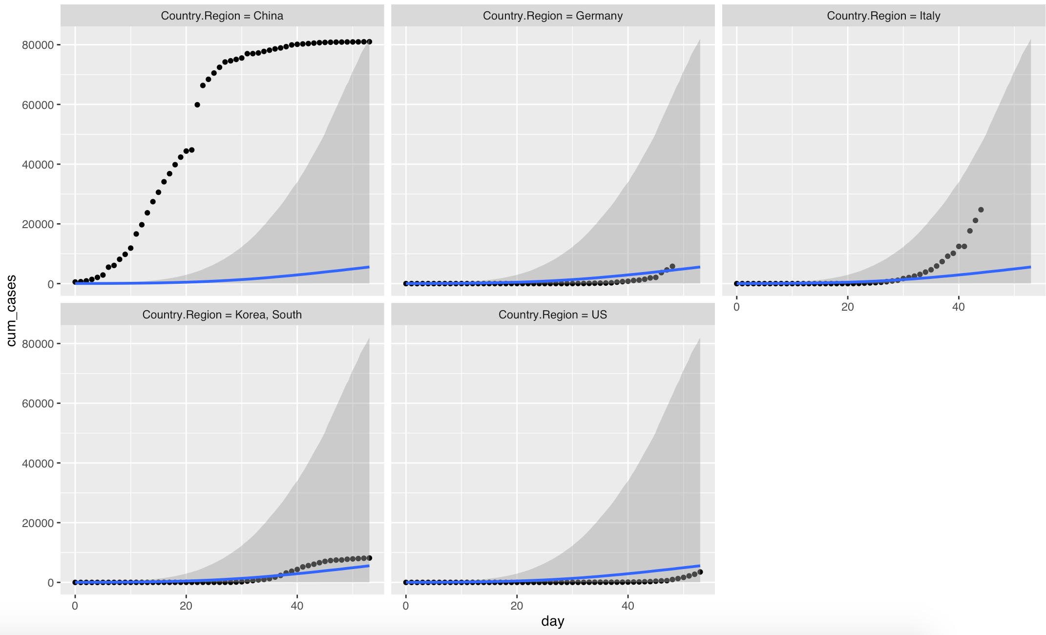
conditions <- make_conditions(case_counts, "Country.Region")
plot(
conditional_effects(
modmult2,
conditions = conditions,
re_formula = NULL
),
points = TRUE,
facet_arg = list(scales = "free")
)
This runs with only a couple of divergences for me (around ~3 divergences; the model runs slooooooow, though). However, the fit seems not so different from what you have posted. The parameters are obviously fairly correlated – especially, logk and logdelay. I’m afraid the (unsatisfactory) answer here could be that the folk theorem of statistical computing comes into play here: the model is probably not so great… :/ But maybe I’m missing something…