Hello,
I’m trying to replicate the examples in the textbook “Causal Inference for Statistics, Social and Biomedical Sciences” by Guido Imbens and Donald Rubin using Stan (obvs!). One of their examples is giving me trouble :( I provide the code to replicate what I did at the end of the post, after a short description of the problem for those not familiar with the methodology in the book.
For those not familiar with the book:
Not surprisingly, the book advocates the use of the Rubin Causal Model (RCM) that uses the potential outcomes framework. For those who don’t know what this is, the RCM for the case of a binary treatment W_i \in \{0,1\} associates two outcomes to each individual i. One for the case the individual was treated, Y_i(1), the other for the case she wasn’t, Y_i(0). We of course only observe one of these two potential outcomes for each individual depending on her treatment assignment
The treatment effect for individual i is \tau_i :=Y_i(1) - Y_i(0), and the average treatment effect is \mathbb{E}[\tau_i]. The crux of this framework is that it clearly turns the problem of causal inference into a missing data problem. In fact, most causal inference methods can be mapped into different ways to impute the missing outcomes.
Simple example succesfully replicated
Chapter 8 of the book is about how to impute the missing potential outcomes by modeling the joint distribution of the missing and observed data and then impute the missing outcomes from the posterior predictive distribution of the missing outcomes. Their examples use the famous Lalonde data set which consists of the outcomes of a labor training experiment. The outcome of interest is the earnings of those involved in the experimnent a year after it concluded.
Here’s the code for the simple case–which I can replicate–in which both potential outcomes are modelled as normal
With normal priors on the mean and inverse gamma on the standard deviations, this case can be solved analytically and they do that in the book. Below is the Stan program for this model.
     data {
      int<lower=1> N;             // number of observations
      real<lower=0> Y_obs[N];     // observed outcome
      int<lower=0, upper=1> W[N]; // treatment assignment indicator
    }
    parameters {
      real mu_0;      // mean vector of potential ouctome of untreated
      real mu_1;      // mean vector of potential ouctome of treated
      real<lower=0> sigma_0;
      real<lower=0> sigma_1;
    }
    model {
      // priors
      mu_0 ~ normal(0, 100);
      mu_1 ~ normal(0, 100);
      sigma_0 ~ cauchy(0, 10);
      sigma_1 ~ cauchy(0, 10);
      // likelihood
      for (i in 1:N) {
        if (W[i] == 0) {
          Y_obs[i] ~ normal(mu_0, sigma_0);
        }
        else if (W[i] == 1) {
          Y_obs[i] ~ normal(mu_1, sigma_1);
        }
      }
    }
    generated quantities {
      vector[N] Y_0;
      vector[N] Y_1;
      vector[N] tau_individual;
      real tau;
      for (i in 1:N) {
        if (W[i] == 1) {
          Y_1[i] = Y_obs[i];
          Y_0[i] = normal_rng(mu_0, sigma_0);  // impute midding outcome
        }
        if (W[i] == 0) {
          Y_0[i] = Y_obs[i];
          Y_1[i] = normal_rng(mu_1, sigma_1);  // impute missing outcome
        }
        // compute treatment effect for individual i
        tau_individual[i] = Y_1[i] - Y_0[i];
      }
      tau = mean(tau_individual);
    }
Here’s how I run it in R
# install.packages("devtools")
# devtools::install_github("jjchern/lalonde") # contains the dataset
library(lalonde)
library(data.table)

library(rstan)
options(mc.cores = parallel::detectCores())
rstan_options(auto_write = TRUE)

## the experiment data
nswDT = data.table(lalonde::nsw_dw)

## prepare list od data for Stan
data_stan = list(
N = nrow(nswDT),
Y_obs = nswDT$re78,  ## earnings after experiment
W = nswDT$treat)

## compile stan model
fit.stan = stan(file = "normal-model.stan", data = data_stan)
tau = extract(fit.stan, "tau")[[1]]
mean(tau)
sd(tau)
qplot(tau)
Here’s the histogram of the treatment effects

Beautiful.
They also extend this model by parametrizing the mean using individual’s observables, \mu_0 = X\beta_0 and \mu_1 = X\beta_1. I can also replicate that. Let’s move now to the problematic example.
The problem: Two stage model of potential outcomes
The earnings data contains a lot of zeroes as can be seen here
library(ggplot2)
ggplot(nswDT, aes(x=re74)) + geom_histogram() + facet_grid(~treat)
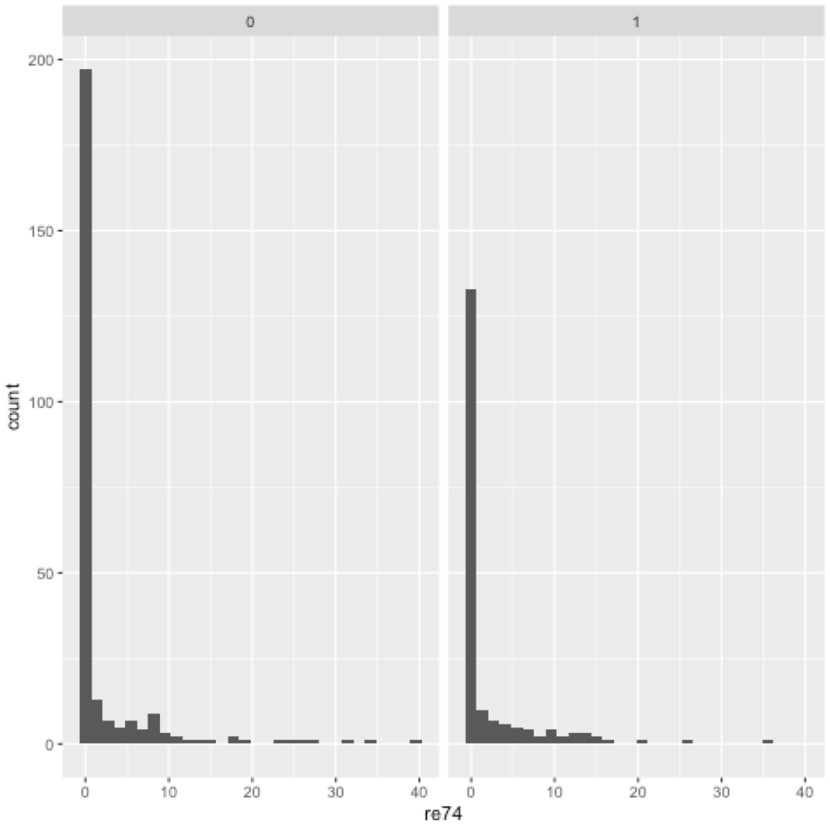
They propose to model the potential outcomes, Y_i(0) and Y_i(1), with a two stage model: a logit that generates the zeroes and a lognormal distribution for the outcomes if they are not zero.
First stage:
Second stage:
and similarly for Y_i(1) with corresponding parameters (\gamma_1, \beta_1, \sigma_1).
Here’s how I wrote this in Stan,
   data {
      int<lower=1> N;               /* number of observations */
      int K;                        /* number of covariates */
      real<lower=0> Y_obs[N];
      int<lower=0, upper=1> W[N];   /* treatment assignment indicator*/
      matrix[N, K] X;               /* matrix of covariates */
    }
    parameters {
      vector[K] gamma_0;            /* params of Y_0 > 0 */
      vector[K] gamma_1;            /* params of Y_1 > 0 */
      vector[K] beta_0;             /* params of Y_0 mean */
      vector[K] beta_1;             /* params of Y_1 mean */
      real<lower=0> sigma_0;
      real<lower=0> sigma_1;
    }
    model {
      // priors
      beta_0 ~ normal(0, 100);
      beta_1 ~ normal(0, 100);
      gamma_0 ~ normal(0, 100);
      gamma_1 ~ normal(0, 100);
      sigma_0 ~ cauchy(0, 10);
      sigma_1 ~ cauchy(0, 10);
      // outcomes model
      for (i in 1:N) {
        if (W[i] == 0) {            /* observe Y_0 */
          // likelihood of the observed Y_0[i]
          if (Y_obs[i] == 0) {
            0 ~ bernoulli_logit(X[i] * gamma_0);
          }
          else if (Y_obs[i] > 0){
            1 ~ bernoulli_logit(X[i] * gamma_0);
            Y_obs[i] ~ lognormal(X[i] * beta_0, sigma_0);
          }
        }
        else if (W[i] == 1){        /* observe Y_1 */
          // likelihood of the observed Y_1[i]
          if (Y_obs[i] == 0) {
            0 ~ bernoulli_logit(X[i] * gamma_1);
          }
          else if (Y_obs[i] > 0) {
            1 ~ bernoulli_logit(X[i] * gamma_1);
            Y_obs[i] ~ lognormal(X[i] * beta_1, sigma_1);
          }
        }
      }
    }
    generated quantities {
      vector[N] Y_0;
      vector[N] Y_1;
      real Y0is0;
      real Y1is0;
      real tau;
      vector[N] tau_individual;
      // generate the "Science" matrix by drawing from
      // the missing data distribution
      for (i in 1:N) {
        if (W[i] == 1) {
          Y_1[i] = Y_obs[i];
          // draw bernoulli_logit to see if Y_0 is zero
          Y0is0 = bernoulli_logit_rng(X[i] * gamma_0);
          if (Y0is0 == 0)
            Y_0[i] = lognormal_rng(X[i] * beta_0, sigma_0);
          else
            Y_0[i] = 0;
        }
        if (W[i] == 0) {
          Y_0[i] = Y_obs[i];
          // draw bernoulli to see if Y_1 is zero
           Y1is0 = bernoulli_logit_rng(X[i] * gamma_1);
          if (Y1is0 == 0)
            Y_1[i] = lognormal_rng(X[i] * beta_1, sigma_1);
          else
            Y_1[i] = 0;
        }
        // compute treatment effect for individual i
        tau_individual[i] = Y_1[i] - Y_0[i];
      }
      tau = mean(tau_individual);
    }
And here is how I run it in R
## prepare covariates
nswDT[, `:=`(re74is0 = as.integer(re74==0),
                 re75is0 = as.integer(re75==0))]

names.covariates = c("age", "education", "married", "nodegree",
                                   "black", "re74", "re74is0", "re75", "re75is0")

data_stan.covariates = list(
      N = nrow(nswDT),
      K = 10,
      Y_obs = nswDT$re78,
      W = nswDT$treat,
      X = as.matrix(nswDT[, c(intercept = 1, .SD), .SDcols=names.covariates]))

## run Stan
fit.ts = stan('two-stage-model.stan', data=data_stan.covariates)

tau
I get that the average treatment effect is \tau = 0.114 (0.48), while in the book they report 1.57 (0.75), much more in line with the simpler model.

Is there something I’m doing wrong? Has anyone used Stan to work on causal inference problems using the potential outcomes framework and can share an example?
Thank you!
Edit:
The coefficients I get are almost identical to the ones reported in the book. Below are two tables with posterior means and standard deviations for all the model’s coefficients. The first one is from the book, the second one from my model.
The coefficients are almost identical with two major exceptions. First, the coefficients corresponding to the variables indicating zero earnings in the past years have flipped signs. After checking, I’m almost certain the authors defined those variables in the opposite way they intended. That would not change anything substantive about the treatment effects, only flip the sign on the coefficients of those variables.
Second, the constants on the first stage logit for Y_i(0) and Y_i(1) reported in the book are \gamma_0 = 2.54 (1.49) and \gamma_1 = 2.54+0.68 (2.49) = 3.22, whereas I get \gamma_0=3.11 (1.62) and \gamma_1 = 2.71.
Book coefficients:

My coefficients (in the same order as in the book’s table):
