# Model over-estimates inflation. Why?
**URL:** https://discourse.mc-stan.org/t/model-over-estimates-inflation-why/27355
**Category:** Modeling
**Tags:** brms
**Created:** [May 4, 2022, 3:00pm UTC](https://discourse.mc-stan.org/t/model-over-estimates-inflation-why/27355 "2022-05-04T15:00:15Z")
**Posts on this page:** 18
**Page:** 1
### Author:  [@jd\_c](https://discourse.mc-stan.org/u/jd_c)
#### Post date: [May 4, 2022, 3:00pm UTC](https://discourse.mc-stan.org/t/model-over-estimates-inflation-why/27355/1 "2022-05-04T15:00:15Z")
Over on this lengthy [thread](https://discourse.mc-stan.org/t/discrepancy-between-y-and-yrep-in-pp-check-how-bad-is-it/27193/18), I suggested an implementation of a custom family in brms for a zero-one-midpoint-inflated beta model for slider scale data. The reasons for having such a thing would be 1) slider scale data really does appear this way - people hate it, are neutral, or love it, 2) generally slider scale data has multiple responses per person, and it would be nice to model the different inflation components using correlated varying effects for person, 3) this would all be super handy and convenient in brms.
I have started a new topic, because the original was slightly off topic and got rather lengthy. I had more time to think about it, and now I have some questions.
Defining a custom response distribution wouldn’t seem so difficult, as there is already a `zero_one_inflated_beta` in brms. I would think that you could simply add a line for the midpoint inflation to the currently implemented `zero_one_inflated_beta`, like this:
```nohighlight
stan_funs <- "
real zero_one_mid_inflated_beta_lpdf(real y, real mu, real phi,
real zoi, real coi, real mdi) {
row_vector[2] shape = [mu * phi, (1 - mu) * phi];
if (y == 0) {
return bernoulli_lpmf(1 | zoi) + bernoulli_lpmf(0 | coi);
} else if (y == 1) {
return bernoulli_lpmf(1 | zoi) + bernoulli_lpmf(1 | coi);
} else if (y == 0.5) {
return bernoulli_lpmf(1 | mdi);
} else {
return bernoulli_lpmf(0 | zoi) + bernoulli_lpmf(0 | mdi) + beta_lpdf(y | shape[1], shape[2]);
}
}
"
```
Now in the previous topic that I linked to, I implemented it like this:
```nohighlight
stan_funs <- "
real zero_one_mid_inflated_beta_lpdf(real y, real mu, real phi,
real zoi, real coi, real mdi) {
row_vector[2] shape = [mu * phi, (1 - mu) * phi];
if (y == 0) {
return bernoulli_lpmf(1 | zoi) + bernoulli_lpmf(0 | coi);
} else if (y == 1) {
return bernoulli_lpmf(1 | zoi) + bernoulli_lpmf(1 | coi);
} else if (y == 0.5) {
return bernoulli_lpmf(1 | mdi) + bernoulli_lpmf(0 | mdi);
} else {
return bernoulli_lpmf(0 | zoi) + bernoulli_lpmf(0 | mdi) + beta_lpdf(y | shape[1], shape[2]);
}
}
"
```
which seems like a mistake to include the `+ bernoulli_lpmf(0 | mdi)` in the midpoint inflation line.
However, the latter does a much better job at estimating the midpoint inflation than the former! Why??
Here is fully reproducible code to implement the first one as shown above, with results and posterior predictive checks:
```nohighlight
library(brms)
#proportion of zero-one inflation (zoi) = 200/800 = 0.25
#proportion of zoi that are ones (coi) = 100/200 = 0.5
#mid-point inflation (mdi) = 100/800 = 0.125
#mean of the beta distribution is 0.5
y <- c(rep(0, 100), rbeta(500, 1, 1), rep(0.5, 100), rep(1, 100))
hist(y,breaks=50)
d1 <- cbind(y)
d1 <- data.frame(d1)
str(d1)
## TRY 1
zero_one_mid_inflated_beta <- custom_family(
"zero_one_mid_inflated_beta", dpars = c("mu", "phi", "zoi", "coi", "mdi"),
links = c("logit", "identity", "identity", "identity", "identity"),
lb = c(0, 0, 0, 0, 0), ub = c(1, NA, 1, 1, 1),
type = "real"
)
stan_funs <- "
real zero_one_mid_inflated_beta_lpdf(real y, real mu, real phi,
real zoi, real coi, real mdi) {
row_vector[2] shape = [mu * phi, (1 - mu) * phi];
if (y == 0) {
return bernoulli_lpmf(1 | zoi) + bernoulli_lpmf(0 | coi);
} else if (y == 1) {
return bernoulli_lpmf(1 | zoi) + bernoulli_lpmf(1 | coi);
} else if (y == 0.5) {
return bernoulli_lpmf(1 | mdi);
} else {
return bernoulli_lpmf(0 | zoi) + bernoulli_lpmf(0 | mdi) + beta_lpdf(y | shape[1], shape[2]);
}
}
"
stanvars <- stanvar(scode = stan_funs, block = "functions")
m1 <- brm(y ~ 1, data=d1, family = zero_one_mid_inflated_beta, stanvars = stanvars, cores = 4)
m1
posterior_predict_zero_one_mid_inflated_beta <- function(i, prep, ...) {
zoi <- get_dpar(prep, "zoi", i)
coi <- get_dpar(prep, "coi", i)
mdi <- get_dpar(prep, "mdi", i)
mu <- get_dpar(prep, "mu", i = i)
phi <- get_dpar(prep, "phi", i = i)
hu <- runif(prep$ndraws, 0, 1)
one_or_zero <- runif(prep$ndraws, 0, 1)
mid <- runif(prep$ndraws, 0, 1)
ifelse(hu < zoi & mid > mdi,
ifelse(one_or_zero < coi, 1, 0),
ifelse(mid < mdi, 0.5, rbeta(prep$ndraws, shape1 = mu * phi, shape2 = (1 - mu) * phi))
)
}
pp_check(m1, type='hist')
```


And here is the second implementation that would seem incorrect but does a better job:
```nohighlight
## TRY 2
zero_one_mid_inflated_beta <- custom_family(
"zero_one_mid_inflated_beta", dpars = c("mu", "phi", "zoi", "coi", "mdi"),
links = c("logit", "identity", "identity", "identity", "identity"),
lb = c(0, 0, 0, 0, 0), ub = c(1, NA, 1, 1, 1),
type = "real"
)
stan_funs <- "
real zero_one_mid_inflated_beta_lpdf(real y, real mu, real phi,
real zoi, real coi, real mdi) {
row_vector[2] shape = [mu * phi, (1 - mu) * phi];
if (y == 0) {
return bernoulli_lpmf(1 | zoi) + bernoulli_lpmf(0 | coi);
} else if (y == 1) {
return bernoulli_lpmf(1 | zoi) + bernoulli_lpmf(1 | coi);
} else if (y == 0.5) {
return bernoulli_lpmf(1 | mdi) + bernoulli_lpmf(0 | mdi);
} else {
return bernoulli_lpmf(0 | zoi) + bernoulli_lpmf(0 | mdi) + beta_lpdf(y | shape[1], shape[2]);
}
}
"
stanvars <- stanvar(scode = stan_funs, block = "functions")
m2 <- brm(y ~ 1, data=d1, family = zero_one_mid_inflated_beta, stanvars = stanvars, cores = 4)
m2
posterior_predict_zero_one_mid_inflated_beta <- function(i, prep, ...) {
zoi <- get_dpar(prep, "zoi", i)
coi <- get_dpar(prep, "coi", i)
mdi <- get_dpar(prep, "mdi", i)
mu <- get_dpar(prep, "mu", i = i)
phi <- get_dpar(prep, "phi", i = i)
hu <- runif(prep$ndraws, 0, 1)
one_or_zero <- runif(prep$ndraws, 0, 1)
mid <- runif(prep$ndraws, 0, 1)
ifelse(hu < zoi & mid > mdi,
ifelse(one_or_zero < coi, 1, 0),
ifelse(mid < mdi, 0.5, rbeta(prep$ndraws, shape1 = mu * phi, shape2 = (1 - mu) * phi))
)
}
pp_check(m2, type='hist')
```


In both cases the midpoint inflation is over-estimated. However, the first implementation has a much greater over-estimation.
Why is that? It seems like the first one would be the correct implementation. ??
---
### Author:  [@jsocolar](https://discourse.mc-stan.org/u/jsocolar)
#### Post date: [May 4, 2022, 6:26pm UTC](https://discourse.mc-stan.org/t/model-over-estimates-inflation-why/27355/2 "2022-05-04T18:26:00Z")
In your option 1, the line for `else if (y == 0.5)` is missing the lp contribution from NOT being in the zoi state. That is, it’s missing `bernoulli_lpmf(0 | zoi)`
---
### Author:  [@jd\_c](https://discourse.mc-stan.org/u/jd_c)
#### Post date: [May 4, 2022, 6:40pm UTC](https://discourse.mc-stan.org/t/model-over-estimates-inflation-why/27355/3 "2022-05-04T18:40:53Z")
Ooohh… so wouldn’t it also be missing `bernoulli_lpmf(0 | mdi)` from the zero and one inflation lines?
---
### Author:  [@jd\_c](https://discourse.mc-stan.org/u/jd_c)
#### Post date: [May 4, 2022, 6:46pm UTC](https://discourse.mc-stan.org/t/model-over-estimates-inflation-why/27355/4 "2022-05-04T18:46:53Z")
Ok, so this implementation successfully recovers the inflation from the simulated data.
```nohighlight
## TRY 4
zero_one_mid_inflated_beta <- custom_family(
"zero_one_mid_inflated_beta", dpars = c("mu", "phi", "zoi", "coi", "mdi"),
links = c("logit", "identity", "identity", "identity", "identity"),
lb = c(0, 0, 0, 0, 0), ub = c(1, NA, 1, 1, 1),
type = "real"
)
stan_funs <- "
real zero_one_mid_inflated_beta_lpdf(real y, real mu, real phi,
real zoi, real coi, real mdi) {
row_vector[2] shape = [mu * phi, (1 - mu) * phi];
if (y == 0) {
return bernoulli_lpmf(1 | zoi) + bernoulli_lpmf(0 | coi) + bernoulli_lpmf(0 | mdi);
} else if (y == 1) {
return bernoulli_lpmf(1 | zoi) + bernoulli_lpmf(1 | coi) + bernoulli_lpmf(0 | mdi);
} else if (y == 0.5) {
return bernoulli_lpmf(1 | mdi) + bernoulli_lpmf(0 | zoi);
} else {
return bernoulli_lpmf(0 | zoi) + bernoulli_lpmf(0 | mdi) + beta_lpdf(y | shape[1], shape[2]);
}
}
"
stanvars <- stanvar(scode = stan_funs, block = "functions")
m4 <- brm(y ~ 1, data=d1, family = zero_one_mid_inflated_beta, stanvars = stanvars, cores = 4)
m4
posterior_predict_zero_one_mid_inflated_beta <- function(i, prep, ...) {
zoi <- get_dpar(prep, "zoi", i)
coi <- get_dpar(prep, "coi", i)
mdi <- get_dpar(prep, "mdi", i)
mu <- get_dpar(prep, "mu", i = i)
phi <- get_dpar(prep, "phi", i = i)
hu <- runif(prep$ndraws, 0, 1)
one_or_zero <- runif(prep$ndraws, 0, 1)
mid <- runif(prep$ndraws, 0, 1)
ifelse(hu < zoi & mid > mdi,
ifelse(one_or_zero < coi, 1, 0),
ifelse(mid < mdi, 0.5, rbeta(prep$ndraws, shape1 = mu * phi, shape2 = (1 - mu) * phi))
)
}
pp_check(m4, type='hist')
```


So it seems it was missing `bernoulli_lpmf(0 | zoi)` from the midpoint inflation line as @jsocolar mentioned and `bernoulli_lpmf(0 | mdi)` from the zero and one inflation lines.
Does that look correct? It seems to work properly.
---
### Author:  [@jsocolar](https://discourse.mc-stan.org/u/jsocolar)
#### Post date: [May 4, 2022, 7:01pm UTC](https://discourse.mc-stan.org/t/model-over-estimates-inflation-why/27355/5 "2022-05-04T19:01:41Z")
> [@jd\_c](#):
>
> Ooohh… so wouldn’t it also be missing `bernoulli_lpmf(0 | mdi)` from the zero and one inflation lines?
Not quite. The way you set up the conditionals, you first ask “are we in the zero-one-inflation state?” Everything that _is_ in this state can ignore all the contributions associated with what happens when you are not in this state (for example, it isn’t relevant whether you’re in the .5-inflated state or not given that you are in the zero inflation state. Then, you want to ask, _conditional on NOT being in the zero-one-inflated state_, what’s the probability that you’re in the .5 inflation state. Your .5 inflation probability is interpretable as the probability of being a .5 conditional on not being a zero or a one.
If you want you could flip it around. You could first ask whether or not you’re in the .5-inflation state, and conditional on not being in the .5 inflation state you could ask whether you’re in the zero-one inflation state. Or you could first ask whether or not you’re in a zero-one-0.5-inflated state, and sift through all of that stuff.
But as you’ve written it, the first two cases don’t need the `bernoulli_lpmf(0 | mdi)` for the same reason that the last two lines don’t need anything to do with `bernoulli_lpmf(0 | coi)`.
What you cannot do is write the model so that the zero-inflation parameter, one-inflation parameter, and 0.5-inflation parameter all give _unconditional_ probabilities of being in the associated state without some additional structure to encode that these events are mutually exclusive.
---
### Author:  [@jd\_c](https://discourse.mc-stan.org/u/jd_c)
#### Post date: [May 4, 2022, 7:17pm UTC](https://discourse.mc-stan.org/t/model-over-estimates-inflation-why/27355/6 "2022-05-04T19:17:48Z")
> [@jsocolar](#):
>
> Not quite. The way you set up the conditionals, you first ask “are we in the zero-one-inflation state?” Everything that _is_ in this state can ignore all the contributions associated with what happens when you are not in this state (for example, it isn’t relevant whether you’re in the .5-inflated state or not given that you are in the zero inflation state. Then, you want to ask, _conditional on NOT being in the zero-one-inflated state_ , what’s the probability that you’re in the .5 inflation state. Your .5 inflation probability is interpretable as the probability of being a .5 conditional on not being a zero or a one.
Thanks! I guess I will have to think about this a bit more. I think I see what you are saying, that makes sense, but if I just include `bernoulli_lpmf(0 | zoi)` in the midpoint inflation line, without `bernoulli_lpmf(0 | mdi)` in the zero-one inflation lines, then the model gets the zero and one inflation correct but over-estimates the midpoint inflation:
```no-highlight
stan_funs <- "
real zero_one_mid_inflated_beta_lpdf(real y, real mu, real phi,
real zoi, real coi, real mdi) {
row_vector[2] shape = [mu * phi, (1 - mu) * phi];
if (y == 0) {
return bernoulli_lpmf(1 | zoi) + bernoulli_lpmf(0 | coi);
} else if (y == 1) {
return bernoulli_lpmf(1 | zoi) + bernoulli_lpmf(1 | coi);
} else if (y == 0.5) {
return bernoulli_lpmf(1 | mdi) + bernoulli_lpmf(0 | zoi);
} else {
return bernoulli_lpmf(0 | zoi) + bernoulli_lpmf(0 | mdi) + beta_lpdf(y | shape[1], shape[2]);
}
}
"
```

So something is still amiss.
It worked when I included `bernoulli_lpmf(0 | mdi)` in the zero-one inflation lines. Why is that?
---
### Author:  [@jsocolar](https://discourse.mc-stan.org/u/jsocolar)
#### Post date: [May 4, 2022, 7:19pm UTC](https://discourse.mc-stan.org/t/model-over-estimates-inflation-why/27355/7 "2022-05-04T19:19:01Z")
Are you sure it overestimates the midpoint inflation? Recall that the estimate is the midpoint inflation _conditional on not being a zero or a 1_
---
### Author:  [@jd\_c](https://discourse.mc-stan.org/u/jd_c)
#### Post date: [May 4, 2022, 7:28pm UTC](https://discourse.mc-stan.org/t/model-over-estimates-inflation-why/27355/8 "2022-05-04T19:28:40Z")
Oh, right! So in that case it is spot on! 100 out of 600 obs, when the zero and ones are removed, which is approx 0.17. Thanks!
In that case, the code for `posterior_predict` needs work as well.
Just curious, the last code seems to give accurate results for just the proportion of 0.5 values - why? It is of course incorrect for the inflation conditional on not being a zero or a 1.
---
### Author:  [@jsocolar](https://discourse.mc-stan.org/u/jsocolar)
#### Post date: [May 4, 2022, 7:33pm UTC](https://discourse.mc-stan.org/t/model-over-estimates-inflation-why/27355/9 "2022-05-04T19:33:00Z")
If the probabilities of 0, 1, and 0.5 are sufficiently small, then it will be approximately true that `p(0 AND 1 AND 0.5) = 0 ~= p(0) * p(1) * p(0.5)`, and treating these events as though they’re independent will get you close.
---
### Author:  [@jd\_c](https://discourse.mc-stan.org/u/jd_c)
#### Post date: [May 4, 2022, 7:37pm UTC](https://discourse.mc-stan.org/t/model-over-estimates-inflation-why/27355/10 "2022-05-04T19:37:36Z")
thanks for the help!! I will look at the `posterior_predict` code and then post the all the corrected model code here, later.
---
### Author:  [@jd\_c](https://discourse.mc-stan.org/u/jd_c)
#### Post date: [May 10, 2022, 3:35pm UTC](https://discourse.mc-stan.org/t/model-over-estimates-inflation-why/27355/11 "2022-05-10T15:35:55Z")
I coded a slightly more thorough simulation and updated the model code to reflect the correction above and also to use logit links for the inflation parameters, so that they could be modeled as well. I made a simulation where the probabilities of choosing 0, 0.5, or 1 are influenced by treatment group. The code for the data and plotting is below.
```nohighlight
library(brms)
library(ggplot2)
###simulate zomib data
trt <- c(rep(0, 1000), rep(1, 1000))
n <- length(trt)
a_zoi <- 0.25
b_zoi <- 0.2
a_coi <- 0.5
b_coi <- 0.3
a_mdi <- 0.1
b_mdi <- 0.3
a_b <- 0.5
b_b <- 0.25
zoi <- a_zoi + trt*b_zoi
coi <- a_coi + trt*b_coi
mdi <- a_mdi + trt*b_mdi
phi <- 2
mu <- a_b + trt*b_b
shape1 <- mu * phi
shape2 <- (1 - mu) * phi
y <- vector("numeric", n)
y <- ifelse(
rbinom(n, 1, zoi)==1,
rbinom(n, 1, coi),
ifelse( rbinom(n, 1, mdi)==1, 0.5, rbeta(n, shape1, shape2))
)
d1 <- cbind(trt,y)
d1 <- data.frame(d1)
d1$trt.f <- factor(d1$trt)
str(d1)
table((d1$y==0 | d1$y==1)[d1$trt==0])
table((d1$y==1)[d1$trt==0])
table((d1$y==0.5)[d1$trt==0])
hist(d1$y, breaks=100)
ggplot(d1, aes(y, fill = trt.f)) +
geom_histogram(alpha=0.75, position="identity", binwidth = 0.01) +
scale_fill_manual(values = c("#0275d8", "#f0ad4e")) +
theme(panel.grid.major.y = element_blank(), panel.grid.minor.y = element_blank()) +
theme(panel.grid.major.x = element_blank(), panel.grid.minor.x = element_blank()) +
theme(panel.background = element_rect(fill = "white")) +
theme(axis.line.x = element_line(colour = "black")) +
theme(axis.line.y = element_line(colour = "black"))
```

As can be seen in the histogram, for trt==1, there is increased probability of neutral (0.5) and 1 choices, as well as a shift toward higher values.
Now define the custom response distribution for a zero-one-mid-inflated beta model and run the model:
```nohighlight
###define custom response distribution for zomib in brms
zero_one_mid_inflated_beta <- custom_family(
"zero_one_mid_inflated_beta", dpars = c("mu", "phi", "zoi", "coi", "mdi"),
links = c("logit", "identity", "logit", "logit", "logit"),
lb = c(0, 0, 0, 0, 0), ub = c(1, NA, 1, 1, 1),
type = "real"
)
stan_funs <- "
real zero_one_mid_inflated_beta_lpdf(real y, real mu, real phi,
real zoi, real coi, real mdi) {
row_vector[2] shape = [mu * phi, (1 - mu) * phi];
if (y == 0) {
return bernoulli_lpmf(1 | zoi) + bernoulli_lpmf(0 | coi);
} else if (y == 1) {
return bernoulli_lpmf(1 | zoi) + bernoulli_lpmf(1 | coi);
} else if (y == 0.5) {
return bernoulli_lpmf(1 | mdi) + bernoulli_lpmf(0 | zoi);
} else {
return bernoulli_lpmf(0 | zoi) + bernoulli_lpmf(0 | mdi) + beta_lpdf(y | shape[1], shape[2]);
}
}
"
stanvars <- stanvar(scode = stan_funs, block = "functions")
###run zomib model
m.zomib <- brm(bf(y ~ trt.f, zoi ~ trt.f, coi ~ trt.f, mdi ~ trt.f),
data=d1, family = zero_one_mid_inflated_beta, stanvars = stanvars, cores = 4)
m.zomib
```

Now, define the posterior predict function in brms so that we can run `pp_check()`
```nohighlight
###define posterior predict function in brms for posterior predictive checks. run pp_check
posterior_predict_zero_one_mid_inflated_beta <- function(i, prep, ...) {
zoi <- get_dpar(prep, "zoi", i)
coi <- get_dpar(prep, "coi", i)
mdi <- get_dpar(prep, "mdi", i)
mu <- get_dpar(prep, "mu", i = i)
phi <- get_dpar(prep, "phi", i = i)
hu <- runif(prep$ndraws, 0, 1)
one_or_zero <- runif(prep$ndraws, 0, 1)
mid <- runif(prep$ndraws, 0, 1)
ifelse(hu < zoi,
ifelse(one_or_zero < coi, 1, 0),
ifelse(mid < mdi & hu > zoi, 0.5, rbeta(prep$ndraws, shape1 = mu * phi, shape2 = (1 - mu) * phi))
)
}
pp_check(m.zomib, type='hist')
pp_check(m.zomib, ndraws=30)
```


Looks good. Now compare to a zero-one-inflated beta model for the same data:
```nohighlight
###compare to zoib model
m.zoib <- brm(bf(y ~ trt.f, zoi ~ trt.f, coi ~ trt.f), data=d1, family = zero_one_inflated_beta, cores = 4)
m.zoib
pp_check(m.zoib, type='hist')
pp_check(m.zoib, ndraws=30)
```


As can be seen from the posterior predictive checks, the zoib model doesn’t capture the mid-point inflation, while the zomib model does.
The recovery of the simulation parameters can be checked for each model in this code:
```nohighlight
###compare recovery of parameters from the sim for the two models
##check to see if sim parameters were recovered by the zomib model
s.zomib <- as_draws_df(m.zomib)
#a_zoi, zero-one inflation for trt=0, was 0.25
a_zoi.zomib <- plogis(s.zomib$b_zoi_Intercept)
mean(a_zoi.zomib)
quantile(a_zoi.zomib, c(0.025, 0.975))
#b_zoi, change in zero-one inflation for trt=1 vs trt=0, was 0.2
b_zoi.zomib <- plogis(s.zomib$b_zoi_Intercept + s.zomib$b_zoi_trt.f1) - plogis(s.zomib$b_zoi_Intercept)
mean(b_zoi.zomib)
quantile(b_zoi.zomib, c(0.025, 0.975))
#a_coi, one inflation for trt=0, was 0.5
a_coi.zomib <- plogis(s.zomib$b_coi_Intercept)
mean(a_coi.zomib)
quantile(a_coi.zomib, c(0.025, 0.975))
#b_coi, change in one inflation for trt=1 vs trt=0, was 0.3
b_coi.zomib <- plogis(s.zomib$b_coi_Intercept + s.zomib$b_coi_trt.f1) - plogis(s.zomib$b_coi_Intercept)
mean(b_coi.zomib)
quantile(b_coi.zomib, c(0.025, 0.975))
#a_mdi, midpoint inflation conditional on not being a zero or one, for trt=0, was 0.1
a_mdi.zomib <- plogis(s.zomib$b_mdi_Intercept)
mean(a_mdi.zomib)
quantile(a_mdi.zomib, c(0.025, 0.975))
#b_mdi, change in midpoint inflation for trt=1 vs trt=0, was 0.3
b_mdi.zomib <- plogis(s.zomib$b_mdi_Intercept + s.zomib$b_mdi_trt.f1) - plogis(s.zomib$b_mdi_Intercept)
mean(b_mdi.zomib)
quantile(b_mdi.zomib, c(0.025, 0.975))
#a_b, mean for trt=0 for beta distribution, was 0.5
a_b.zomib <- plogis(s.zomib$b_Intercept)
mean(a_b.zomib)
quantile(a_b.zomib, c(0.025, 0.975))
#b_b, change in mean for beta distribution for trt=1 vs trt=0, was 0.25
b_b.zomib <- plogis(s.zomib$b_Intercept + s.zomib$b_trt.f1) - plogis(s.zomib$b_Intercept)
mean(b_b.zomib)
quantile(b_b.zomib, c(0.025, 0.975))
##compare sim parameters to those of the zoib model
s.zoib <- as_draws_df(m.zoib)
#a_zoi, zero-one inflation for trt=0, was 0.25
a_zoi.zoib <- plogis(s.zoib$b_zoi_Intercept)
mean(a_zoi.zoib)
quantile(a_zoi.zoib, c(0.025, 0.975))
#b_zoi, change in zero-one inflation for trt=1 vs trt=0, was 0.2
b_zoi.zoib <- plogis(s.zoib$b_zoi_Intercept + s.zoib$b_zoi_trt.f1) - plogis(s.zoib$b_zoi_Intercept)
mean(b_zoi.zoib)
quantile(b_zoi.zoib, c(0.025, 0.975))
#a_coi, one inflation for trt=0, was 0.5
a_coi.zoib <- plogis(s.zoib$b_coi_Intercept)
mean(a_coi.zoib)
quantile(a_coi.zoib, c(0.025, 0.975))
#b_coi, change in one inflation for trt=1 vs trt=0, was 0.3
b_coi.zoib <- plogis(s.zoib$b_coi_Intercept + s.zoib$b_coi_trt.f1) - plogis(s.zoib$b_coi_Intercept)
mean(b_coi.zoib)
quantile(b_coi.zoib, c(0.025, 0.975))
#a_b, mean for trt=0 for beta distribution, was 0.5
a_b.zoib <- plogis(s.zoib$b_Intercept)
mean(a_b.zoib)
quantile(a_b.zoib, c(0.025, 0.975))
#b_b, change in mean for beta distribution for trt=1 vs trt=0, was 0.25
b_b.zoib <- plogis(s.zoib$b_Intercept + s.zoib$b_trt.f1) - plogis(s.zoib$b_Intercept)
mean(b_b.zoib)
quantile(b_b.zoib, c(0.025, 0.975))
```
I will not post all of the output, but just note that the zomib model recovers all the simulation parameters quite well. The zoib model recovers the parameters (other than mid-point inflation, for which there is no parameter in the zoib model) quite well, except for the change in mu for the beta distribution for the trt==1 group, where it underestimates 0.19 (0.16 - 0.22) the programmed 0.25 value, while the zomib model recovers it.
So far so good. Here is where I get a little bit unsure.
Now, define posterior\_epred for brms, so that we can use `conditional_effects`.
```nohighlight
posterior_epred_zero_one_mid_inflated_beta <- function(prep) {
with(prep$dpars, zoi * coi + (mdi * 0.5)*(1 - zoi) + mu * ( (1 - zoi) * (1 - mdi) ) )
}
conditional_effects(m.zomib)
```

Now let’s compare this to the zoib model.
```nohighlight
conditional_effects(m.zoib)
```
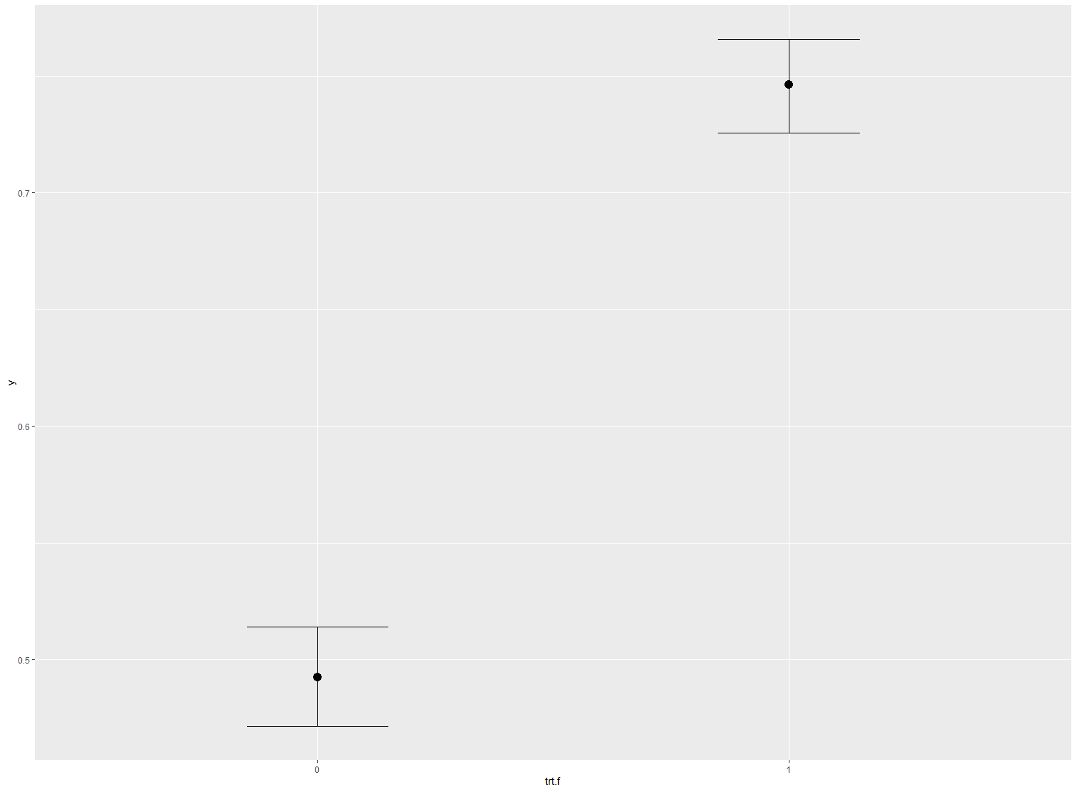
Hmmm, they don’t look so different. Perhaps that is expected, as the zoib model simply seems to average over the midpoint inflation, so maybe it isn’t unexpected that the predictions would be so different.
Now try to define the log-likelihood for the zomib model, so that we can compare the two models via LOO.
```nohighlight
###define log likelihood in brms to use with LOO. run loo()
log_lik_weight <- function(x, i, prep) {
weight <- prep$data$weights[i]
if (!is.null(weight)) {
x <- x * weight
}
x
}
log_lik_zero_one_mid_inflated_beta <- function(i, prep) {
zoi <- get_dpar(prep, "zoi", i)
coi <- get_dpar(prep, "coi", i)
mdi <- get_dpar(prep, "mdi", i)
if (prep$data$Y[i] %in% c(0, 1)) {
out <- dbinom(1, size = 1, prob = zoi, log = TRUE) +
dbinom(prep$data$Y[i], size = 1, prob = coi, log = TRUE)
} else if (prep$data$Y[i] %in% c(0.5)) {
out <- dbinom(1, size = 1, prob = mdi, log = TRUE) +
dbinom(0, size = 1, prob = zoi, log = TRUE)
} else {
phi <- get_dpar(prep, "phi", i)
mu <- get_dpar(prep, "mu", i)
args <- list(shape1 = mu * phi, shape2 = (1 - mu) * phi)
out <- dbinom(0, size = 1, prob = zoi, log = TRUE) +
dbinom(0, size = 1, prob = mdi, log = TRUE) +
do_call(dbeta, c(prep$data$Y[i], args, log = TRUE))
}
log_lik_weight(out, i = i, prep = prep)
}
loo(m.zomib, m.zoib, cores=1)
```

Now that does seem a bit strange. According to LOO the zomib model is much worse, but as we saw above, the posterior predictive plots and the proper recovery of the simulation parameters indicated that it was much better (in addition, it is the generative model for this data).
It makes me think that I have made an error in the log-likelihood code (and maybe also in the posterior epred code? as I would have thought to see more of difference between treatment groups)? @avehtari@paul.buerkner anyone else? @Solomon
---
### Author:  [@avehtari](https://discourse.mc-stan.org/u/avehtari)
#### Post date: [May 17, 2022, 12:31pm UTC](https://discourse.mc-stan.org/t/model-over-estimates-inflation-why/27355/12 "2022-05-17T12:31:47Z")
> [@jd\_c](#):
>
> Now that does seem a bit strange. According to LOO the zomib model is much worse, but as we saw above, the posterior predictive plots and the proper recovery of the simulation parameters indicated that it was much better (in addition, it is the generative model for this data).
> It makes me think that I have made an error in the log-likelihood code (and maybe also in the posterior epred code?
I guess this is due to comparing continuos density vs discrete probability for observations 0.5, and that is not valid in general. See CV-FAQ [Can cross-validation be used to compare different observation models / response distributions / likelihoods?](http://mc-stan.org/loo/articles/online-only/faq.html#differentmodels) and [Is it a problem to mix discrete and continuous data types?](http://mc-stan.org/loo/articles/online-only/faq.html#is-it-a-problem-to-mix-discrete-and-continuous-data-types-). Easiest way to make the comparison valid, would be to discretize both predictive distributions and compute probabilities within intervals (integrate the continuous density over intervals to get probabilities)
---
### Author:  [@jd\_c](https://discourse.mc-stan.org/u/jd_c)
#### Post date: [May 17, 2022, 12:41pm UTC](https://discourse.mc-stan.org/t/model-over-estimates-inflation-why/27355/13 "2022-05-17T12:41:26Z")
Ahh ok, thanks!
> [@avehtari](#):
>
> Easiest way to make the comparison valid, would be to discretize both predictive distributions and compute probabilities within intervals
Is there an example (code) somewhere of how to do this? Thanks!
---
### Author:  [@jsocolar](https://discourse.mc-stan.org/u/jsocolar)
#### Post date: [May 17, 2022, 1:02pm UTC](https://discourse.mc-stan.org/t/model-over-estimates-inflation-why/27355/14 "2022-05-17T13:02:23Z")
For what it’s worth, I really don’t think you need cross-validation here to decide which model is better; both domain expertise and the posterior predictive check speak pretty loudly in this case. If you do really need cross-validation for some reason, then @avehtari’s solution based on discretization is really smart (no surprise there), but I think an additional caution is warranted: The results will be sensitive to how finely you discretize, and in the limit of very fine discretization the middle-inflated likelihood will always be preferred as long as there is at least one observation that is exactly 0.5 (as intervals get small, the probability mass associated with this observation will approach zero in the not-middle-inflated model but will approach some finite value in the middle-inflated model). So you need to choose the discretization carefully to reflect something about the degree of precision that you care about in your predictions.
---
### Author:  [@jd\_c](https://discourse.mc-stan.org/u/jd_c)
#### Post date: [May 17, 2022, 1:23pm UTC](https://discourse.mc-stan.org/t/model-over-estimates-inflation-why/27355/15 "2022-05-17T13:23:51Z")
> [@jsocolar](#):
>
> For what it’s worth, I really don’t think you need cross-validation here to decide which model is better; both domain expertise and the posterior predictive check speak pretty loudly in this case.
Good point!
> [@jsocolar](#):
>
> The results will be sensitive to how finely you discretize
I was wondering about this myself, and that is why I was asking if there was some code.
But that is a really good point about whether cross-validation is even needed at all here. This is a pretty narrow use case (at least I can’t think off the top of my head of an example other than slider scale data), and it should be fairly obvious when the mid-point inflation is needed in the model.
I might look more into it at some point if @avehtari has some example code, but otherwise might not worry too much about it at this point.
I guess finally, it would be great if @paul.buerkner or anyone else, @jsocolar , could take a look at the `posterior_epred` [above](https://discourse.mc-stan.org/t/model-over-estimates-inflation-why/27355/11) and pasted below again for convenience.
```no-highlight
posterior_epred_zero_one_mid_inflated_beta <- function(prep) {
with(prep$dpars, zoi * coi + (mdi * 0.5)*(1 - zoi) + mu * ( (1 - zoi) * (1 - mdi) ) )
}
conditional_effects(m.zomib)
```
The logic seems correct and inline with what the function appears to do in brms with the prep function, but I would have guessed a bit more of a difference between the zoib and zomib models based on the difference in the estimate for `trt.f1` in the model summary… (again, see the post I linked above for full results and conditional effects plots).
---
### Author:  [@avehtari](https://discourse.mc-stan.org/u/avehtari)
#### Post date: [May 17, 2022, 1:28pm UTC](https://discourse.mc-stan.org/t/model-over-estimates-inflation-why/27355/16 "2022-05-17T13:28:36Z")
@jsocolar’s answer is excellent and I agree with that
---
### Author:  [@avehtari](https://discourse.mc-stan.org/u/avehtari)
#### Post date: [May 17, 2022, 1:31pm UTC](https://discourse.mc-stan.org/t/model-over-estimates-inflation-why/27355/17 "2022-05-17T13:31:10Z")
> [@jd\_c](#):
>
> I might look more into it at some point if @avehtari has some example code
Sorry no. There are some cases where the choice of intervals is natural, but as @jsocolar’s answer implies it’s possible that there is no natural discretization here.
---
### Author:  [@jd\_c](https://discourse.mc-stan.org/u/jd_c)
#### Post date: [May 17, 2022, 1:39pm UTC](https://discourse.mc-stan.org/t/model-over-estimates-inflation-why/27355/18 "2022-05-17T13:39:50Z")
Ok, thanks @avehtari . I agree with @jsocolar , it’s likely not so necessary anyway. Originally I was trying to implement all of the brms functionality as in the Custom Response Distribution vignette for brms, but since comparison to the other type of model that would be used for this data (zoib model) likely can be pretty obviously done with `pp_check` and not so easily (or necessary) with cross-validation, I’m not going to worry about it.
I appreciate the responses. I’ve learned a lot in this attempt at implementing a zomib model in brms. I think I’ll be pretty much done once posterior\_epred is confirmed.