Posterior estimates of rate and shape of gamma distribution are dependent

I have two concerns:

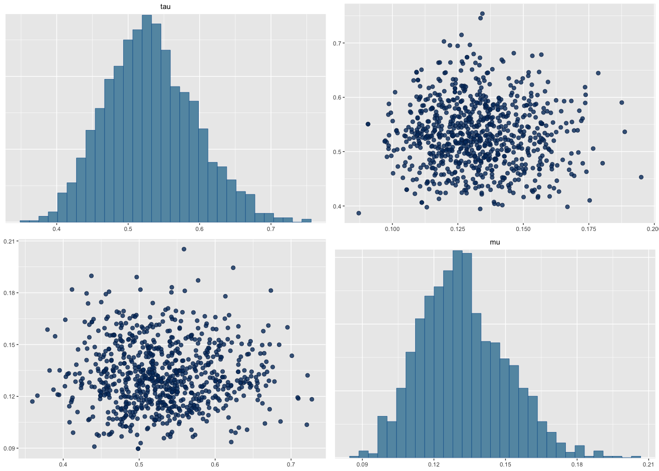
  1. When reporting the estimates of rate and shape, both show similar pattern, which is not very informative. I would prefer some other parametrization which provides orthogonal estimates.

  2. If I recall correctly, the stan prior recommendation list recommends independent priors. Sure, I can set up a gamma model with independent rate and shape priors, but the data then introduce the dependence pattern. Is that not an issue for the sampler? Or, does the sampler use some different implicit parametrization under the hood?

In any case, all of the popular parameter transformations (log rate/shape, scale, mean, mode, std) do not manage to remove the dependence.

What works rather well is parametrization in terms of log scale and log of the geometric mean, but it’s difficult to use this to construct priors because I need to compute inverse digamma function.

For reference here is the model code I am primarily using:

data {
    int<lower=0> N; 
    vector<lower=0>[N] y;
}parameters {
    real b;
    real k;
}model {
 y~gamma(exp(k),exp(b));
}

I’ve tried different priors and I’ve also run a fake data simulation with identical results.

1 Like

I don’t think that is possible with the Gamma distribution. The Fisher information matrix seems to be

   |  trigamma(alpha) | -1/beta        |
N  | ---------------- | -------------- |
   | -1/beta          | alpha / beta^2 |

and I don’t see a substitution that would make that diagonal.

I think it would be better to say there are a bunch of independent priors on the list. That does not mean that if what you believe about the rate depends on what you believe about the shape that you shouldn’t express your prior as f(shape) * f(rate | shape). But it is often difficult for people to express forms of dependence explicitly, so they usually just specify their priors marginally and accept the fact that the posterior distribution has a little less dependence than it ideally should. If you have a decent amount of data, the distortion is pretty negligible.

1 Like

Just for the information. I computed the off-diagonal element of fisher matrix for Gamma distribution parametrized by log geometric mean and log scale and it is indeed equal to zero suggesting that log geometric mean and log scale provide orthogonal parametrization.

For those interested, here is my STAN implementation of inverse digamma function:

functions{
    vector invdigamma(vector x){
        vector[num_elements(x)] y; vector[num_elements(x)] L;
        for (i in 1:num_elements(x)){
            if (x[i]==digamma(1)){ 
                y[i]=1;
            }else{ if (x[i]>=-2.22){
                y[i]=(exp(x[i])+0.5);
            }else{
                y[i]=1/(x[i]-digamma(1));
        }}}
        L=digamma(y)-x;
        while (min(L)>10^-12){
            y=y-L ./trigamma(y);
            L=digamma(y)-x;
        }
        return y;}
    real invdigammaR(real x){
        real y; real L;
        if (x==digamma(1)){ 
            y=1;
        }else{ if (x>=-2.22){
            y=(exp(x)+0.5);
        }else{
            y=1/(x-digamma(1));
        }}
        L=digamma(y)-x;
        while (L>10^-12){
            y=y-L ./trigamma(y);
            L=digamma(y)-x;
        }
        return y;
    }
}
5 Likes

Good to know

1 Like

Hey, I was wondering if you kept investigating this topic.

I’ve got a manuscript ready that investigates the orthogonal parametrization of gamma, Weibull and inverse Gaussian distribution and of some of their extensions. It got rejected by “Communications in Statistics – Theory and Methods” because it lacked application (i.e. analysis of empirical data). All other suitable journals, that I’m aware of, require applications as well. I will have to add it to the manuscript. This takes time.

So far I made parameter recovery experiments with hierarchical gamma distribution with the orthogonal parameterzation. It worked well. You can find the (currently undocumented) code here: GitHub - simkovic/OrthoPar

I’m currently using the following code to compute the inverse gamma function.

real invdigamma(real x){
    real y; real L;
    if (x>=-5.24) y=1/log(1+exp(-x));
    else y=1/(digamma(1)-x);
    L=digamma(y)-x;
    while (fabs(L)>1e-12){
         y=y-L ./trigamma(y);
         L=digamma(y)-x;}
    return y;}

The code I posted previously had mistakes in the formula for computation of starting values. The latest version uses the formulas from Batir (2018) to compute the starting values. These are pretty accurate.

Batir, N. (2018). Inequalities for the inverses of the polygamma functions. Archiv der Mathematik, 110(6):581–589.

4 Likes

I don’t see how the off diagonal goes to 0 with this parameterization. Do you have the derivation?

Thanks for coming back so quickly. I’ll have a look at the resources. This might be very useful in the context of degradation modelling and reliability.
yet I need to understand better what you have done.
Thanks and keep up.

Define Gamma distribution as:
f(Y=y;\rho,\theta)=\frac{1}{\Gamma(\rho) \theta^\rho} y^{\rho - 1} e^{-\frac{y}{\theta}}

and the new parametrization as \gamma=E[\log Y]=\psi(\rho)+\log \theta and \tau=\log(\theta)

Then the diagonal element is

\begin{align} \operatorname{E}_Y \left[ \frac{\partial \log f(Y;\tau,\gamma)}{\partial\tau\ \partial\gamma} \right]&= \operatorname{E}\left[\omega''(\gamma-\tau)(\gamma-\log y)\right] \\ &=\omega''(\gamma-\tau)(\gamma-\operatorname{E}[\log y])\\ &=\omega''(\gamma-\tau)(\gamma-\gamma)\\ &=0 \end{align}

where \omega(\cdot) is the inverse digamma function which is monotonic on \mathcal{R} \rightarrow \mathcal{R}^+.

An intermediate result is \begin{align} \frac{\partial \log f(Y;\gamma,\tau)}{\partial\gamma} = (\log y - \gamma)\omega'(\gamma -\tau)\end{align}.

We use a different derivation strategy in the manuscript and I copied these formulas from my private notes. Let me know if there are any formatting errors.

4 Likes

that is cool thanks for sharing! I’m going to put an issue to add this to the user manual. You could make a Stan case study with your manuscript to show the application.

1 Like

Hi @simkovic ! Very cool parametrization, thanks for sharing it.

Any chance you have a similar derivation for the Weibull distribution? Or the manuscript/preprint published?

I’m fitting a Weibull model but empirical coverage gets hurt due to overestimation of the shape parameter, which seems to be alleviated by orthogonal parametrization (e.g., this paper focusing on modified profile likelihood).

Thanks a lot!

1 Like

If I understood you correctly, the shape parameter is of interest and you need the formula for the orthogonal nuisance parameter. The solution is given in Section 3.4 in the following work:

Cox, D. R., & Reid, N. (1987). Parameter orthogonality and approximate conditional inference. Journal of the Royal Statistical Society: Series B (Methodological), 49(1), 1-18.

1 Like

Thanks a lot!

I was just looking for different (information orthogonal) parameterizations for the Weibull distribution. Of note, the Yang & Xie (2003) paper indicates a typo in the original Cox & Reid derivation for the Weibull case.

Yang, Z., & Xie, M. (2003). Efficient estimation of the Weibull shape parameter based on a modified profile likelihood. In Journal of Statistical Computation and Simulation (Vol. 73, Issue 2, pp. 115–123). Informa UK Limited. https://doi.org/10.1080/00949650215729

TL;DR: Try reparameterizing with the mean and the [untransformed] shape parameter. Could someone please check this?


As a whimsical personal exercise, analogous to the normal I tried reparameterizing the gamma in terms of its mean and [untransformed] scale. It didn’t work, Fisher information off-diagonals were not 0.

On an even greater whim, I tried in terms of its mean and [untransformed] shape. And I think this transformation does orthogonalize the Fisher information. Given that I would imagine this has been tried before, I’d like others to check my work here.

Let the gamma distribution be parameterized by positive shape parameter \alpha and positive scale parameter \beta. The new parameterization is the mean \mu = \alpha\, \beta and untransformed shape \tau = \alpha. For x > 0, this new density is

\frac{\exp{(-x \tau / \mu)}\ x^{\tau - 1}} {(\mu / \tau)^\tau\ \Gamma(\tau) }

and thus its log density is

(\tau - 1) \log{(x)} + \tau (\log{(\tau)} - \log{(\mu)}) - \log{(\Gamma(\tau))} - x\, \tau / \mu,

or, rearranging for clarity,

\mathit{<univariate}\ \mathit{ stuff>} - \tau \log{(\mu)} - x\, \tau / \mu

The off-diagonal Hessian element of this is (x - \mu) / \mu^2. Clearly the (negative) expectation of this is zero.

It’s much harder to find errors when proofreading one’s own work versus proofreading others. Can someone confirm, or correct, this result? If this is confirmed, I would expect it to be a boon for both the OP and the community.

2 Likes

That looks right.

I get higher n_eff with this parameterization than the built in.

functions {
  real johnnys_gamma_lpdf(vector x, real tau, real mu) {
    int N = num_elements(x);
    
    return (tau - 1) * sum(log(x)) + N * tau * (log(tau) - log(mu)) - N * lgamma(tau) - sum(x) * tau / mu;
  }
}
data {
  int<lower=0> N;
  vector[N] x;
}
parameters {
  real<lower=0> mu;
  real<lower=0> tau;
}
model {
  x ~ johnnys_gamma(tau, mu);
}

library(cmdstanr)

mod_gamma <- cmdstan_model("gamma_ortho.stan")

x <- rgamma(100, 0.5, 4)

out <- mod_gamma$sample(
  data = list(N = 100,
              x = x),
  parallel_chains = 4,
  iter_warmup = 400,
  iter_sampling = 400
)
out

library(bayesplot)

out_draws <- out$draws()
mcmc_pairs(out_draws, pars = c("tau", "mu"))

5 Likes